We decided to write a series of posts on a very useful statistical technique called Principal Component Analysis (PCA). In the current post we give a brief explanation of the technique and its implementation in excel. In practice it is less important to know the computations behind PCA than it is to understand the intuition behind the results. For those who are interested to know the mathematics behind this technique we recommend any multivariate statics book. One book which we really like is Carol Alexander’s Market Risk Analysis Volume 1. This book comes with a free excel addin Matrix.xla that can be used to implement PCA in excel. Alternatively the reader can download this excellent addin for free from http://excellaneous.com/Downloads.html.

The idea of PCA is to find a set of linear combinations of variables that describe most of the variation in the entire data set. For example, we may have a time series of daily changes in interest rate swap rates for the past year. We consider changes in 2y, 3y, 4y, 5y, 7y, 10y, 15y, 20y, 30y swap tenors. Our data set has nine variables in total. With so many variables it may be easier to consider a smaller number of combinations of this original data rather than consider the full data set. This is often called a reduction in the data set’s dimension. Having set the goal of reducing dimension of our data set to a smaller number of factors a simple choice would be to use the average. In our case this would be Average = 1/9*2y+1/9*3y+1/9*4y+1/9*5y+1/9*7y+1/9*10y+1/9*15y+1/9*20y+1/9*30y. Our vector of coefficients C=[1/9, 1/9, 1/9, 1/9, 1/9, 1/9, 1/9, 1/9, 1/9] is called a linear combination. Linear combinations where the sum of squared coefficients equal to 1 are called a standardized linear combinations. PCA finds a set of standardized linear combinations where each individual factor is orthogonal (meaning not correlated). There are as many principal components as there are variables in the original data set but they are ordered in such a way that only a few factors explain most of the original data. The orthogonal factors are computed from the correlation or covariance matrix of the original (sometimes standardized) data.

Let’s walk through an example to gain a better understanding. We start out with daily changes in US swap rates for abovementioned tenors.

We would like to reduce the dimension to as few factors as possible that describe the variability in the data. To run PCA on the data we need to generate a correlation or covariance matrix. We choose to use a covariance matrix in this example.

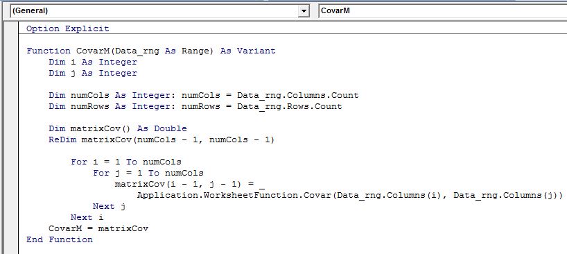
To make the calculations of a covariance matrix easier we use below custom array function that will loop through each data column and calculate pair wise covariance using excels built in COVAR function

We can then use =MEigenvecPow(OurCovarianceMatrix,TRUE) function from the Matrix.xla addin to generate the eigenvector of the covariance matrix. These values are often called loadings. Below are the results for our example.

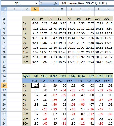
Now it is time for the interpretation of the results. The loading for each factor give us the sensitivity of a particular variable to a 1 unit change in a given factor (principal component). For example, in the above, if the first principal component goes up by 1 then the 2yr swap rate will change by .17 bps, the 5yr will go up but .36bps, and 30yr swap will increase by.35 bps (this is the first column of the matrix). The second column gives us the loadings for the second factor (principal component). In this case, when the second principal component increases by 1, the short end of the curve will increase while the longer end will decrease. This just means that the curve flattens as the second principal component increases. Finally, when the third principal component increases, the short and long end of the curve increases while the middle points of the curve decrease.

When we plot the loadings we can see the data better.

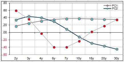
This shows us that the first component captures mostly parallel yield curve moves, the second captures the slope, while the third captures the curvature (butterfly).

So far we spoke about changes in principal components. We would like to know what value they actually take. This is easy; each principal component is a linear combination of the original data and the loadings. So for example, using above data, on 26 Jun2015 the first principal component is equal to 14.70 [.17*4.18 +.25*2.67+.32*3.47 +.36*4.28+.38*5.18+ .38*5.48 +.37*6.02+.36*6.05+.35*6.34]. Calculating a time series of the first three principal components we can see that they are indeed uncorrelated (orthogonal)

Now we would like to answer the obvious question, why did we stop at three principal components in our discussion above. The answer is that three components account for 99.7% of the variation in the data. How can we compute that number? We can use the eigenvalues of our covariance/correlation matrix. To compute these we use MEigenvalPow(OurCovarianceMatrix) from the matrix.xla addin. Below (green row) presents our results.

To assign meaning to these values and compute the percentage of variation that each principal component explains we need to do the following; Take the sum of all eigenvalues. In our example the sum across the green row is 155.41. We can now divide the first eigenvalue by 155.41 to get 90.4%. This means the first principal component explains 90.4% of the variation in the data. The second component captures 8.7% [13.57/155.41]. We can see that in total the first three principal components explain approximately 99.7% of the variation in the data. Adding more factors doesn’t add to our understanding of the data.

We wish to come back to our main point that we mentioned at the start. PCA is used to represent the original data as a function of a reduced number of factors. In our case that means each change in yield for a chosen swap tenor is a function of three factors. So, for example, on any given day the change in 30yr swap is a given by its loadings times the principal components. On 26 June 2015 the first principal component was 14.70, the second principal component was -1.65 and the third was 1.71. From above table of loadings we see that the loadings of 30yr tenor for the first three principal components are .35, -.45, .35. Taking the sum of products we get 6.48 [(14.7*.35)+(-1.65*-.45)+.(1.71*.35)]. This means that we can expect the 30yr swap rate to increase by 6.48 bps given the change in the first three principal components that we witnessed. The actual change on June 26 2015 was 6.34bps.

In this post we tried to present an intuitive explanation of Principal Component Analysis. In follow up posts we will discuss the many uses of PCA in managing risk, modelling asset prices, and trading.

Some useful resources:

1) Market Risk Analysis Volume 1 by Carol Alexander: http://www.amazon.com/Market-Analysis-Quantitative-Methods-Finance/dp/0470998008/ref=sr_1_2?s=books&ie=UTF8&qid=1435483909&sr=1-2&keywords=market+risk+analysis