A logit model is a type of a binary choice model. We use a logistic equation to assign a probability to an event. We define a logistic cumulative density function as:

which is equivalent to

Another property of the logistic function is that:

The first derivative of the logistic function, which we will need when deriving the coefficients of our model, with respect to z is:

In a logistic regression model we set up the equation below:

In this set up using ordinary least squares to estimate the beta coefficients is impossible so we must rely on maximum likelihood method.

Under the assumption that each observation of the dependent variable is random and independent we can derive a likelihood function. The likelihood that we observe our existing sample under the assumption of independence is simply the product of the probability of each observation.

Our likelihood function is:

Where Y is either 0 or 1. We can see that when Y =1 then we have P and when Y=0 we have (1-P)

The aim of the maximum likelihood method is to derive the coefficients of the model that maximize the likelihood function. It is much easier to work with the log of the likelihood function.

From calculus we know that a functions maximum is at a point where its first derivative is equal to zero. Therefore our approach is to take the derivative of the log likelihood function with respect to each beta and derive the value of betas for which the first derivative is equal to zero. This cannot be done analytically unfortunately so we must resolve to using a numerical method. Fortunately for us the log likelihood function has nice properties that allows us to use Newton’s method to achieve this.

Newton’s method is easiest to understand in a univariate set up. It is a numerical method for finding a root of a function by successively making better approximations to the root based on the functions gradient (first derivative).

As a quick example we know that we can approximate a function using first order Taylor series approximation.

where Xc is the current estimate of the root. By setting the function to zero we get

This means that in each step of the algorithm we can improve on an initial guess for x using above rule. Same principles apply to a multivariate system of equations:

Here x is a vector of x values and J is the Jacobian matrix of first derivatives evaluated at vector xc and F is the value of the function evaluated at using latest estimates of x.

Coming back to our logistic regression problem what we are trying to do is to figure out a combination of beta parameters for which our log likelihood function is at a maximum which is equivalent to deriving the set of coefficients where the first derivatives of the likelihood function are all equal to zero. We will do this by using Newton’s numerical method. In the notation from above F is the collection of our log likelihood function’s derivatives with respect to each beta and J is the Hessian matrix of second order partial derivatives of the likelihood function with respect to each beta.

It is a little tedious but necessary to work out these derivatives analytically so we can feed them into our spreadsheet.

Lets restate the log likelihood function once more:

And lets remember that in our case Pi is modeled as:

We will list all the steps in the calculations for those who wish to double check the work

First lets calculate

and via chain rule

Therefore

Also,

and via chain rule

Now we can work through the derivative of our likelihood function.

The derivative of Y with respect to beta (highlighted in red) is equal to zero so we are left with:

Now we can substitute our calculated derivatives:

Values in red cancel out and we are left with:

Now we need to calculate the Hessian matrix. Remembering that:

we have:

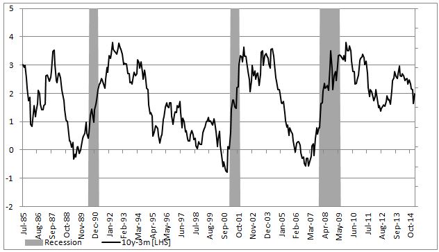
To show an example of how to implement this in excel we will attempt to model the probability of a recession in US (as defined by NBER) with a 3 month lead time. In our set up Y = 1 if US experiences a recession in 3months time and 0 otherwise. Our explanatory variable will be the 10yr3mth treasury curve spread. The yield curve is widely considered to be a leading indicator for economic slowdowns and curve inversion is often considered a sign of a recession.

In the chart below we highlight US recessions in grey while the black line is the yield curve.

The model we are trying to estimate is:

In a spreadsheet we load data on historical recessions in column C and our dependent variable in column D which refers to column C but 3 months ahead. In column E we input 1 which will be our intercept. Column F has historical values for the yield curve. In column G we calculate the probability with the above formula. Our initial guess for betas is zero which we have entered in cell C2 and C3.

In column H we calculate the log likelihood function for each observation. we sum all the values in cell H5. Therefore H5 contains the value of the below formula while each row has a value for each i in the brackets.

Column I calculates the derivative of the likelihood function for each observation with respect to the intercept. Column J calculates the derivative of the likelihood function for each observation with respect to the second beta. The sum of the totals for each column are in cells I2 and I3.

Now we need to calculate the second order derivatives of the likelihood function with respect to each beta. We need 4 in total but remembering that (hessian matrix is symmetric) we only need to calculate 3 columns.

Column K through M calculates the partial derivatives for each row and the sums are reported in a matrix in range J2:K3

Now we finally need to calculate the incremental adjustment to our beta estimates as dictated by the Newton algorithm.

Remember:

We can use Excel’s functions MINVERSE to calculate the inverse of the Hessian matrix and MMULT function to multiply by our Jacobian matrix. Inputting =MMULT(MINVERSE(J2:K3),I2:I3) in range H2:H3 and pressing Ctrl+Shift+Enter since these are array functions we get the marginal adjustment needed.

Finally in G2 we calculate the adjusted intercept beta by subtracting H2 from C2. We do the same for the second beta.

All the calculations shown so far constitute just one iteration of the Newton algorithm. The results so far look like below:

we can copy and paste as values range G2:G3 to C2:C3 to calculate the second iteration of the algorithm

Notice that the log likelihood function has increased. We now have our new estimates in G2:G3. We can copy and paste as values into C2:C3 again. And we should repeat this until the Jacobian matrix is showing zeroes. Once both entries in I2:I3 are zero our log likelihood function is at a maximum.

The algorithm has converged after only 6 iterations and we get below estimates for betas

Overall the model does a poor job of forecasting recessions. The red line shows the probabilities.

In a follow up post we will show how to implement logistic regression in VBA. We will also introduce statistical methods to validate the model and to check for statistical significance of the estimated parameters.

A final note, in this post we wanted to provide a thorough explanation of the logistic regression model and the empirical example we have chosen is too simplistic to be used in practice. However using this approach to model recession probabilities can be very fruitful. Below is an example of a six factor model using the same techniques that forecasts historical recession episodes very well.