In this post we would like to expand on previous PCA post and show you how to build a very useful tool for scenario analysis of a yield curve. The method presented is an implementation of the main results of a paper by Leonardo M. Nogueira “Updating the Yield Curve to Analyst’s Views”. The SSRN link is at the end of the post.

If we find ourselves in a situation where we have a view on a particular point on a yield curve, for example the 2 year swap rate in Australia,  we will probably need to know what the rest of the curve would look like if our view is correct.  So what we need is a method to update the rest of the curve points based on where we think the two year yield is. There are many ways that we can draw a line through a single point so in order to have a sensible estimate for the full curve we need to impose some constraints. In the method that is presented below the constraint that we impose is that the curve is consistent with the main principal components.

The main formula that we will be working with is found on page 5 of the paper that we mentioned.

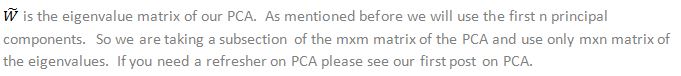
In case of a yield curve mu is set to zero so we are left with:

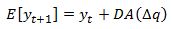
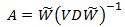
where

To help with the interpretation of the formula let’s put some flesh on our example. Lets work with the Australian yield curve. We have a time series matrix for the following tenors (2y, 3y, 4y, 5y, 7y, 10y, 12y, 15y, 20y, 25y, 30y). We will be working with daily observations for each tenor dating back 3 years. Further, let’s assume we have a view on where 2y and 5y yields are going to be. We want to know what the rest of the curve will look like if we are correct in our assumptions for the two swap rates. To do so we will need to use the first two principal components. If we had a view only on one swap tenor then we can only use the first principal component to derive the full yield curve. The key point is that if we have m tenors (in our case m =11) but only n views (in our case n= 2, ie 2y and 5y swap rates) we can use the first n principal components to derive where all m swap rates are likely to be.

Now we can use our example to help with the interpretation of the arguments of the above formula.

V is a nxm matrix that holds 1 in place for any tenor that we have a view on and 0 otherwise. Again in our example we have eleven tenors with views on only the 2y and 5y swap rate. Therefore in the first row of V we will have the first column set to 1 (because 2y swap rate is the first tenor in our yield curve) and 0 in the rest of the columns. In the second row V will have 1 in the 4th row because that is the placement of our 5y tenor in the yield curve and 0 otherwise.

We can then use excel’s native matrix multiplication and inverse function to derive the expected change in each yield curve tenor. By adding the expected changes to the current yield curve we are left with the expected yield curve.

Excel Implementation:

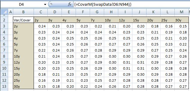
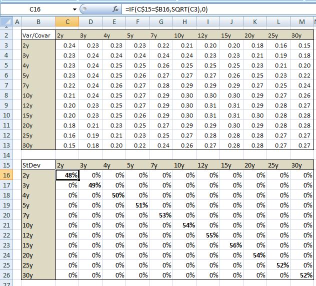
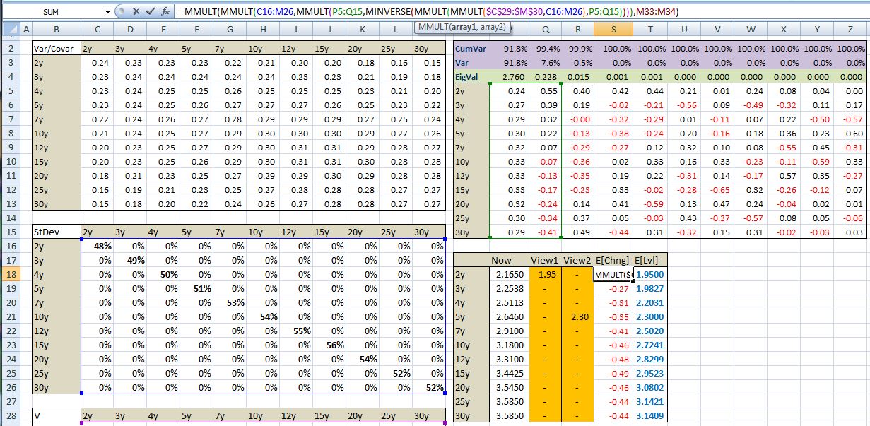
We first need to calculate the variance/covariance matrix of our swap data. We discussed this in our first PCA post with some user defined functions. We do this in range C3:M13

Now we can calculate matrix D by taking the square root of the main diagonal. This is done in range C16:M26

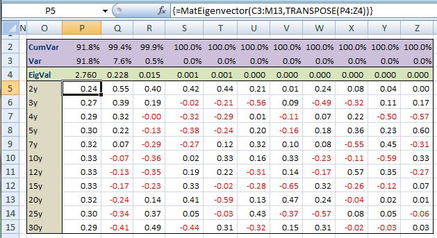
Next we can carry out PCA using matrix.xla add-in that was created by Leonardo Volpi and the Foxes Team (this add-in is no longer supported on the foxes team’s webpage but is available at http://excellaneous.com/. We discussed implementation of PCA using this add-in in our first post on PCA and you can refer to it to see the functions and their uses. The eigenvector is in range P5:Z15

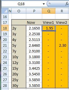
Now we can set up our current yield curve and a range that will hold our forecast for 2y and 5y tenors. In column P we input the current swap rates. In column Q we input our expected value for the 2y tenor. Let’s assume we assume 2y swap rate is going to 1.95%. In column R we input our estimate for the 5y swap rate. Again let’s assume we think the 5y rate is going to 2.30%. It is important to note that with this set up we must have one input in each column.

To review, so far we have our column matrix y, we have our matrix D and we have our eigenvalues which is W hat. We still need matrix V and delta q.

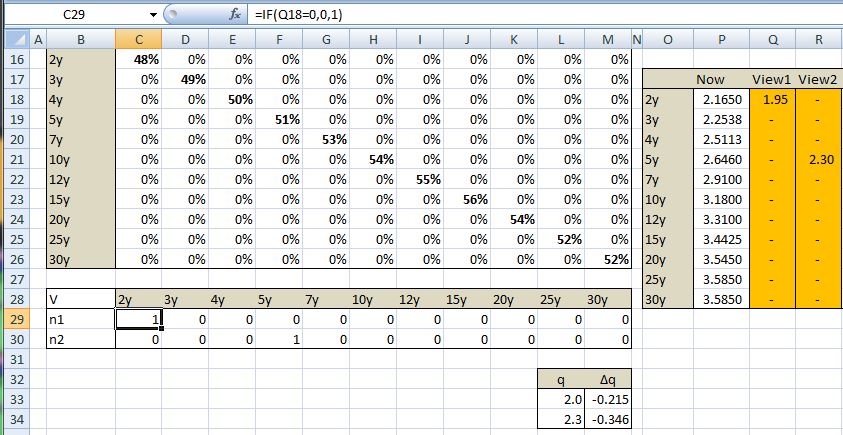
In range C29:M30 we set up matrix V. In range M33:M34 we set up our delta q matrix. Delta q is simply a matrix that holds our expected changes of each tenor (for example, our expected 2y yield of 1.95 less 2.165 current 2y yield yields -.215)

So now we have all the components needed to derive the full yield curve. In range S18:S28 input the formula =MMULT(MMULT(C16:M26,MMULT(P5:Q15,MINVERSE(MMULT(MMULT($C$29:$M$30,C16:M26),P5:Q15)))),M33:M34)

This will calculate

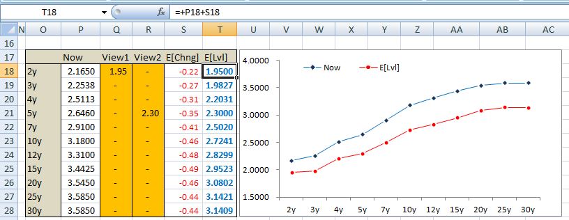
We can then add the results to our current yield curve and we are finished

We can see that the derived curve matches exactly our expected values for the 2y and 5y swap rate and also gives up the rest of the tenors that are consistent with the first two principal components which account for over 99% of the variance in the data.

VBA Implementation:

Above implementation is a touch tedious. We took the long road to help with the exposition of the main results. This same method can be implemented neatly in VBA without all the intermediate calculations in excel. Below is the main function:

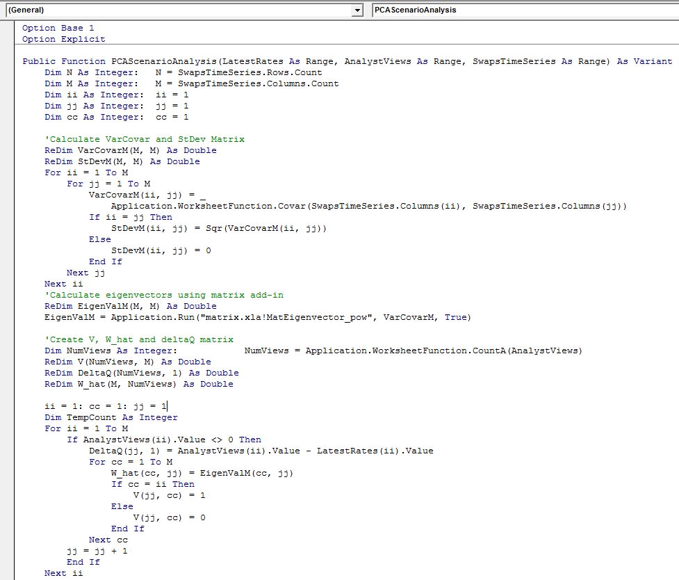
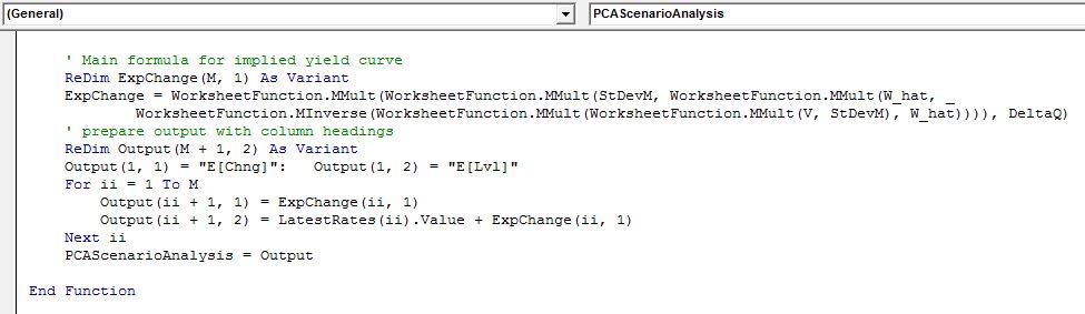
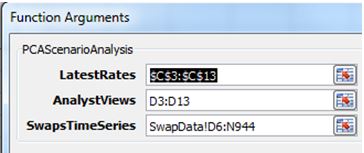
To use the function we need to enter it as an array function by selecting a range 2 columns wide and M+1 rows and then hitting Shift+Ctrl+Enter.

In a spreadsheet we input the function is range E2:F13

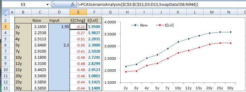
The results agree with our excel implementation earlier.

Final Note:

This method can be used with all yield curves, volatility surfaces and futures curves. A word of caution for macro traders, this approach will not work across asset classes. For instance if you are looking to see what the expected change in USDJPY is given your expectations for SPX and US rates by running this function, you will be disappointed with the results. Main reason this approach does not work is because the variance/covariance matrix is unstable and hence your PCA results will be dubious. We have carried out extensive backtests on this approach across asset classes and without exception results are poor. This approach to scenario analysis works incredibly well on highly correlated time series such as yield curves but may breakdown when there is a regime change. For example, modelling US yield curve with data that only includes history of when Fed was on hold should be made with caution given the likely changes in Fed policy in the near future.

Some useful resources:

1. This is a link to the main paper ~ http://papers.ssrn.com/sol3/papers.cfm?abstract_id=1107653
2. https://quantmacro.wordpress.com/2015/06/28/principal-component-analysis-in-excel-part-i/
3. https://quantmacro.wordpress.com/2015/06/29/principal-component-analysis-part-ii/
4. Market Risk Analysis Volume 1 by Carol Alexander (an excellent source about PCA): http://www.amazon.com/Market-Analysis-Quantitative-Methods-Finance/dp/0470998008/ref=sr_1_2?s=books&ie=UTF8&qid=1435483909&sr=1-2&keywords=market+risk+analysis