I have been on a machine learning MOOCS binge in the last year.  I must say some are really amazing.  The one weakness so far is the treatment of support vector machines (SVM).  It’s a shame really since other popular classification algorithms are covered.  I should mention that there are two exceptions, Andrew Ng’s Machine Learning on Coursera and Statistical Learning course on Stanford’s Lagunita platform.   Both courses miss the mark when it comes to SVM in my opinion.  Andrew Ng watered down the presentation of SVM classifiers compared to his Stanford class notes but he still treated the subject much better than his competitors.  Statistical Learning by Trevor Hastie and Rob Tibshirani was an amazing course but unfortunately SVM was treated somewhat superficially.  I hate to be critical of these two courses since overall they are amazing and I am very grateful to the instructors for making this content available for the masses.

I decided to check out some other online content on SVM and have a stab at presenting the material in a style that is friendly to newbies.  This will be a three part series with today’s post covering the linearly separable hard margin formulation of SVM.  In a second post I will discuss a soft margin SVM. In a final post I will discuss what is commonly referred to as the kernel trick to handle non linear decision boundaries.  I borrow heavily from the authors that I will mention at the end of the post so to add some original content I implement SVM in an excel spreadsheet using Solver.  I find that excel is a great pedagogical tool and hope you agree with me and find the toy model interesting.

The Goal:

In this post I will work with an example in two dimensions so that we can easily visualize the geometry of our classifier.  All the points discussed apply equally in higher dimensions.

We will work with a binary classification problem.  Our features space will consist of 12 observations of x1 and x2 pairs.  In general we will have N observations and P will denote the number of features.  Each data point is labeled as a +1 or a -1.  In the plot I have + for +1 and – for -1.

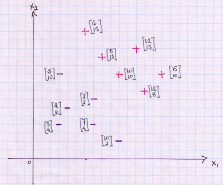
What a linear classifier attempts to accomplish is to split the feature space into two half spaces by placing a hyperplane between the data points.  This hyperplane will be our decision boundary.  All points on one side of the plane will belong to class C1 and all points on the other side of the plane will belong to the second class C2.

Unfortunately there are many ways in which we can place a hyperplane to divide the data.  Below is an example of two candidate hyperplanes for our data sample.

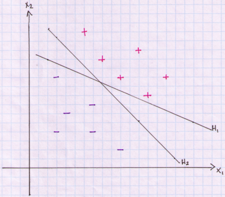
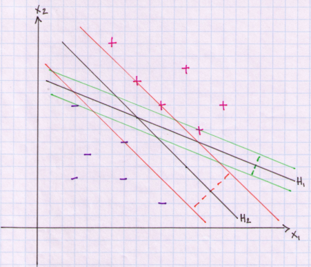
Both H1 and H2 separate the data without making any classification errors.  Points above the line are classified as +1 and points below the line are classified as -1.   A solution to this problem of finding an ‘optimal’ separating hyperplane is to introduce the concept of a margin.  We first select a hyperplane (decision boundary) and then extend two parallel hyperplanes on either side of our decision boundary.  We widen the parallel hyperplanes until we touch one or more of our data points on either side but without allowing any of the points to penetrate the boundaries.  The distance between these parallel hyperplane boundaries is called a margin.  The decision boundary is equidistant from these parallel hyperplanes so that we do not bias our decision in favour of any particular class.  In below plot I show these margins for each decision boundary.  For H1 the parallel hyperplanes are plotted in green.  For H2 the parallel hyperplanes are plotted in orange.  The margins are plotted as dashed lines.  You can see that the margin is larger for H2.  You can think of the margin as the width of a road.  We try to build a straight road that is as wide as possible between the data.  The separating hyperplane is the dividing lane on this road.  We are trying to find the placement of the dividing lane in such a way as to build the widest road that just touches any of our data points.

Defining a hyperplane:

So now that we have our goal set out for us we need to formulate it as a mathematical model.  As we plow along I will take lots of detours to introduce the algebra and geometry.  With each detour I will try to keep us focused on why the concept is important for our problem.

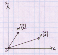
With that in mind let’s begin with a definition of a vector.  A vector can be thought of as a directed line segment.  A vector has a displacement from one point P to another point Q.  A starting point of a vector is called a tail and the ending point is called a head.  If a vector starts from the origin it is called a position vector.  Below is a plot of a two position vectors in two dimensions.

Vectors do not need to have a tail at the origin.  Two vectors are equal if they have the same length and the same direction.  Below we have vector v from O to A and vector w from B to C.

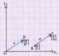
Notice that vector v has displacement of [3,2]. Vector w displacement is also [3,2] and is given simply as the difference of its two components [3,2] = [8-5,3-1] or C-B.

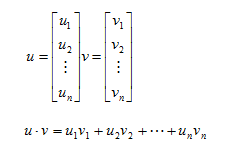
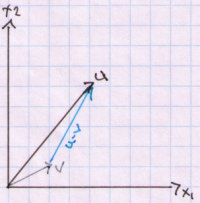
We will use vectors throughout this post.  They are critical to our definition of a hyperplane and we will also use operations on vectors to measure the margin.  Before we move on I want to mention the dot product.  For vectors u and v we define a dot product as:

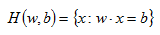
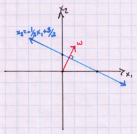
With a definition of a dot product we can now specify an equation for our hyperplane:

In our two dimensional example, x is a vector of [x1,x2].  Vector w and scalar b are the coefficients of our hyperplane.  If for example w=[1,2] and b=3 then our hyperplane is given as:

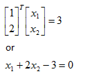
We can rewrite this in the more familiar y=mx+b form by rearanging some terms.

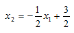
Notice that the slope of the line is given by w1/w2 and the intercept term is given by b/w2.

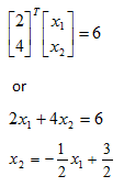
Let’s plot this hyperplane and also include the vector w:

The important thing to note here is that the vector w is perpendicular to our hyperplane.  This means that vector w is at a 90 degree angle to our hyperplane.  This is a very important property, referred to as orthogonality, which we will exploit later when calculating our margin.  The vector w is called the normal vector.

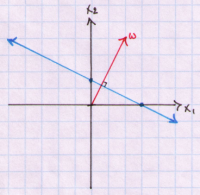
Another important property that will be relevant in our discussion is that multiplying vector w and b by a constant (scalar multiplication) does not change our hyperplane but does extend our normal vector in the original direction.  To see this lets multiply w and b by 2 and plot.  We get:

So now we know that our separating plane will be defined as:

And our decision rule for the model will be:

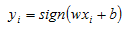
That is, we will assign observation xi to class +1 if wx+b is >0 and assign xi to class -1 if wx+b <0.

Defining the Margin:

Lets again look at a plot of what we are trying to measure, and then I will introduce the bare minimum mathematical definitions for us to be able to compute what we need.  So here goes:

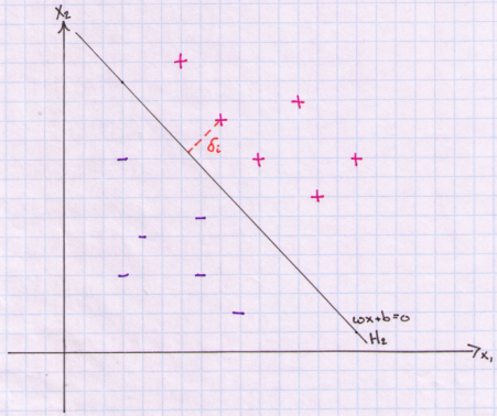
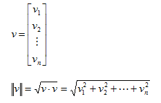
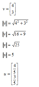
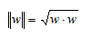
What we need is the distance from a point to our hyperplane.  In the above graph we are interested in the distance delta that is marked as a dashed orange line.  To do so we need to first define the length or magnitude of a vector.   Euclidian length (or norm) of a vector v is defined as the square root of the dot product of v:

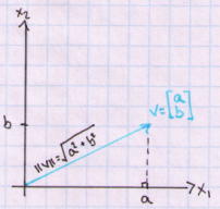
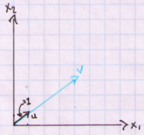
Above result is given by the Pythagoras’ Theorem.  In two dimensions we can see this more clearly. Below I plot vector v=[a,b] and calculate its length from the origin.

Once we have the vector length in hand we can normalize a vector to have unit length.  We simply divide each entry in the vector by the norm.  For example assume we have a vector v= [4,3]. Then unit vector u is:

And finally, let’s define a measure of distance between two vectors.  We can use our measure of length on the difference between two vectors to get its Euclidian distance.

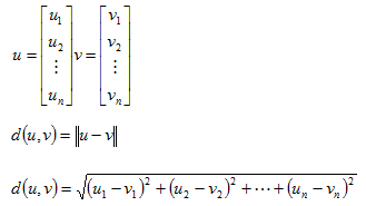
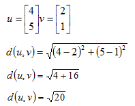
For example, if we have vectors u and v, the distance between them is calculated as:

We now have all the tools we need to calculate the delta value.

In below plot we need to derive the value of delta (dashed orange line).

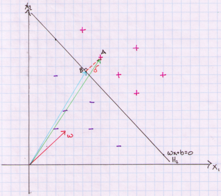
This value of delta is ½ the margin for our decision boundary.  In Euclidean geometry, the shortest distance from a point to a hyperplane is one that is orthogonal to the hyperplane (perpendicular to the line in 2 dimensions). In the plot, delta equals the difference between vector A and vector B.  We know that delta is in the opposite direction of our normal vector (marked in red).  We can use this fact and first compute the pure direction of our normal vector by dividing it by its norm and then multiply it by delta to gives us a vector of length delta and pointing in the direction of the norm.  We then subtract this value from A to arrive at point B on our hyperplane.

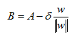
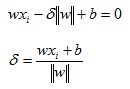
Let’s pause and understand what we did.  We are trying to find a point on the plane that is closest to one of our observations xi.  In the plot we have labeled the point we are trying to compute as B and the data point from where delta is measured is labeled A.  Remember that A is one of our actual observations xi.   We then multiply the length delta by the direction of our normal vector and then subtracted this quantity from our observation xi to end up on the hyperplane at point B.  Once we have point B we can use the fact that any point on our hyperplane produces a value of zero.  Therefore, we can plug in B into the formula for our hyperplane and solve for delta.

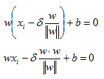
Remember our definition of norm:

Plugging that in and solving for delta we have:

Notice that in the calculations so far we worked with xi that is on the positive side of the decision boundary.  We need to take the absolute value of our delta calculations because when computing the delta from the negative side of the decision boundary we will have a negative value.  However, instead of taking the absolute value we can simply multiply our delta by the class label.  So our final formula becomes:

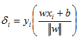
When we are below the decision boundary the value in the bracket is negative and it is multiplied by -1 (our class label).  So we are now dealing with strictly positive deltas.  The above formula is commonly referred to as the geometric margin.

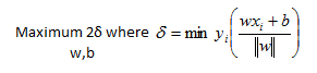
So we now have a formula to compute the distance between any of our observations to our decision boundary.  Lets now remember that delta is defined here as just a single lane of the road (ie, it is half the margin).  Therefore, 2*delta is our margin for any point.  The definition of a margin for the entire sample is simply the minimum margin of all the possible margins in the sample.  And it is important to remember that we are trying to maximize the sample margin.

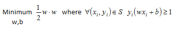
Therefore, our mathematical formulation for the hard margin classifier that we defined at the beginning is:

Optimization Set Up:

Now that we have a mathematical formulation for a maximum margin classifier we have to start thinking about how do we find the w and b that achieve the maximum.  The rest of the post is about simplifying this maximization problem into something that we know we can solve.  To begin with let’s recognize that our definition for the delta as the minimum delta in our sample can be restated as:

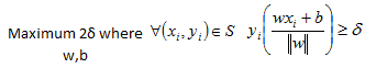
Our objective function remains unchanged and we only changed the way we represent the delta of a sample.  This equation reads as, maximum of margin with respect to w and b where for all xi and yi in our sample the geometric margin is at least equal to delta.

Also, we need to come back to the important point I made earlier about length of w not having any impact on our separating hyperplane.  Remember that if we rescale our normal vector the slope of the hypeplane does not change.  So for convenience let’s set norm of w equal to:

I realize that this is not an obvious choice but if we now solve for delta to get one over length of w and substitute into our maximization formula we can see that this transformed our objective function and the constraints:

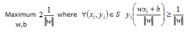
On the right side in the constraints equations please notice we can cancel out the norm of w to leave us with linear constraints.  Linear constraints are much easier to work with so we should be happy with our accomplishments so far.

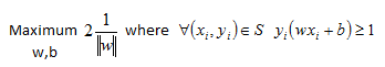
A few final changes are needed to change this maximization problem into something we can easily tackle.  The major problem now is the objective function itself.  The one over w norm is not a nice equation that is easily maximized.  What we can choose to do instead is to minimize the reciprocal of the objective function.

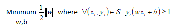
Finally, we can get rid of the square root in the objective function so that we can work with a very well known quadratic programming problem.  We can do this because the square of a function is a monotonic transformation.   In a quadratic programming problem we work with a quadratic objective function subject to linear constraints.  There are many efficient algorithms in most software packages that can solve these problems.

The above problem is what is known as the Primal Form of the optimization problem.

Excel Example 1:

We can now set up a toy example in excel. Below is an example for our data set.

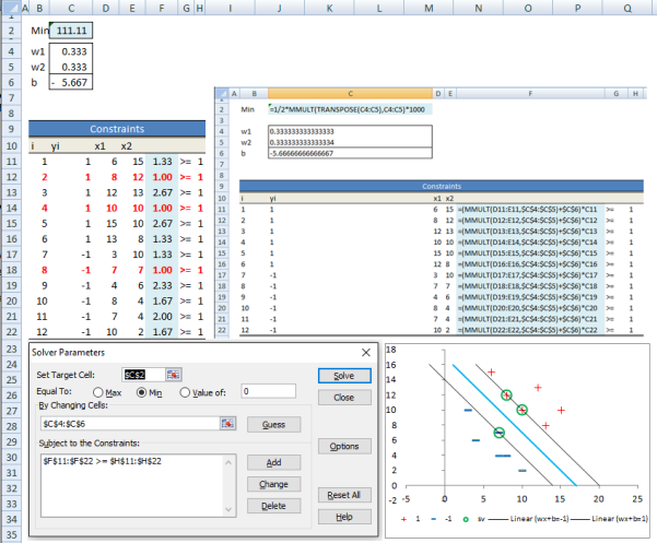
I have included a screenshot with the formulas.  The objective function is in cell C2.  We can add constraints in Solver and then hit <Solve> button.  As can be seen we have 3 data points for which the constraint in the minimization is binding (ie geometric margin is equal to one).  In the plot I highlight these points.  These are called the supporting vectors for our margin classifier.

The Dual Set Up:

To solve the constrained optimization that we have derived so far we can set up a Lagrange function and derive the solution analytically.  Let’s restate the minimization we are trying to compute:

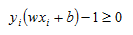
We can rewrite the constraint as:

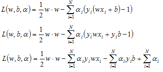
We then multiply all of the constraints by Lagrange multipliers (alphas) and subtract from our objective function:

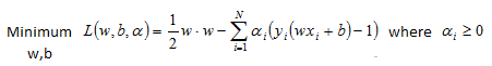
Notice that we are minimizing with respect to w and b but are maximizing with respect to alphas.

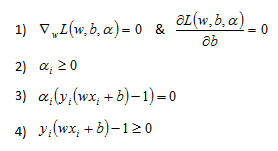
As I mentioned, the quadratic optimization problem is a well studied problem.  A quadratic objective function with linear inequality constraints must satisfy some conditions at the solution.  These conditions are known as KKT conditions and are named after Karush, Kuhn and Tucker who independently derived them.

The KKT conditions are:

First lets expand the Lagrangian to isolate the w and b terms:

Now we can take the derivative of our Lagrange function with respect to the vector w to get:

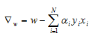
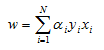
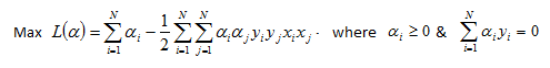
And by setting the result equal to zero and solving for w we get:

Now we can move on to the derivative of the Lagrange formula with respect to b.  We have:

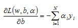
And we again set the result equal to zero:

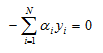
Now let’s substitute these results into the Lagrange function:

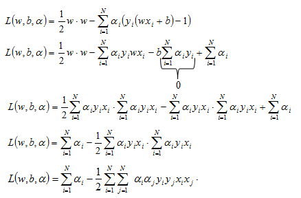
It is important to note that we are now trying to maximize this Lagrange function since it is only a function of alphas.  This is the so-called Dual formulation of the optimization problem.

This can be rewritten in matrix notation as:

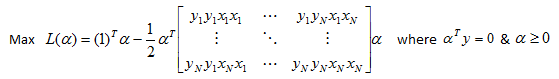
Once we solve for alphas we need to be able to use our classifier.  That means we need the coefficients of our hyperplane.  To get back our coefficients w we can use below equation that we derived earlier:

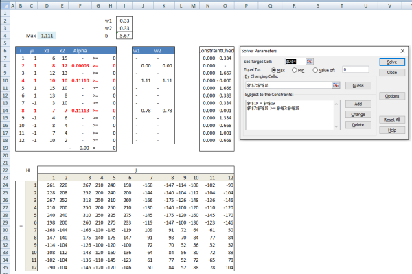
Once we have our w we can use the fact that for any of the support vectors we have:

And we can solve this for our b coefficient:

Now that we have our hyperplane coefficients we can use our classifier to assign any observation xi by plugging it into below equation:

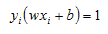
Excel Example 2:

We can set up the maximization problem in a spreadsheet and use Solver to calculate alphas.  Below are the results.  You can see that we have only three alphas that are non zero and they match the support vectors we derived in the Primal example.

I have attached the sheet svm_calcs_example

Sanity Check:

We can perform a quick spot check in R to make sure our results are correct.

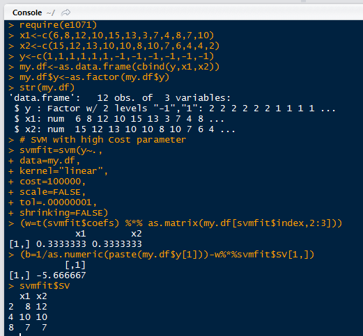
Fortunately we got results that are the same as our excel implementation.

Hope you enjoyed the post. Below are some useful resources.

Useful Resources:

• Idiot’s Guide to SVM from MIT http://web.mit.edu/6.034/wwwbob/svm-notes-long-08.pdf
• Andrew Ng notes http://cs229.stanford.edu/notes/cs229-notes3.pdf
• Lecture 14 on SVM from Yaser Abu-Mostafa at Caltech http://work.caltech.edu/lectures.html
• Thorsten Joachims SVM lecture from Cornell http://svmlight.joachims.org/
• Practical Mathematical Optimization by Jan A Snyman is excellent http://www.springer.com/us/book/9780387243481
• Data Mining by Nong Ye is a good book that has a worked example for the AND function https://www.crcpress.com/Data-Mining-Theories-Algorithms-and-Examples/Ye/p/book/9781439808382
• I used the wife’s Linear Algebra and Its Applications for Algebra review but any textbook will do. https://www.amazon.com/Linear-Algebra-Applications-Updated-CD-ROM/dp/0321287134/ref=sr_1_7?s=books&ie=UTF8&qid=1465859903&sr=1-7