It is commonly known that financial returns exhibit characteristics that are not captured by the widely applied normal and log-normal distributions.  In a series of posts I want to present some flexible distributions that are well suited to model financial returns.  We will work our way through quick modelling exercises in R that show how easy it is to use these alternative distributions.

To begin, I will introduce the Generalized Lambda Distribution (GLD).  There is ample evidence to show that this is an excellent contender for modelling various financial returns.  At the end  of the post I reference two papers that test GLD on FX and Equity returns.

GLD is defined in terms of the inverse cumulative distribution function (cdf):

The only restrictions we have on the parameters is that has to be positive. (This is not unusual – for example, variance in the normal distribution has to be greater than zero).

In R, there is a great package GLDEX that has all the functionality that we need to calibrate the FMKL GLD distribution to data. We will work with SPX data from 2004-2019 and calibrate the distribution parameters to the full data set.

require(quantmod)
require(GLDEX)

SPY_prices <- Ad(getSymbols("SPY", from = "2004-01-01", to = "2019-01-01",
                 auto.assign = FALSE))
returns_xts <- diff(log(SPY_prices), k =1)[-1,]*100
full_sample_fit <- fun.RMFMKL.ml(data = returns_xts)  # MLE fit

fun.plot.fit(full_sample_fit, returns_xts, xlab = 'SPY Return',
             name = 'FMKL.ML', nclass = 75, param.vec = 'fmkl')

We can also check the qq plot to see how well the distribution fits the data.

qqplot.gld(returns_xts, full_sample_fit, 'fmkl', name = 'RMFMKL.ML')

The nice thing is that GLD is already specified as an inverse cumulative normal distribution so we can very easily use it to check Value at Risk (VaR) at a specified level .  For example, VaR at = 0.01 is -3.8%. The 99th percentile of the distribution is 3.06%.

qgl(.01, lambda1= full_sample_fit)
qgl(.99, lambda1= full_sample_fit)

-3.77901522473645
3.05837784742503

One thing the package does not give us is the expected shortfall formula (ES).  ES is the conditional VaR. i.e. the expected loss given that our VaR has been exceeded.

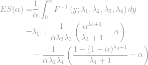
We can implement the function below.

ES_FMKL_GLD <- function(alpha, lambda1, lambda2=NULL, lambda3=NULL, lambda4=NULL){
    if (length(lambda1) > 1) {
        lambda2 <- lambda1[2]
        lambda3 <- lambda1[3]
        lambda4 <- lambda1[4]
        lambda1 <- lambda1[1]
    }
    lambda1 + 1/(alpha*lambda2*lambda3) * ((alpha^(lambda3+1))/(lambda3+1)-alpha) - 
              1/(alpha*lambda2*lambda3) * ((1-(1-alpha)^(lambda4+1))/(lambda4+1) - alpha)
}

Let’s check it against numerical integration:

alpha <- .01
round(ES_FMKL_GLD(alpha, lambda1 = full_sample_fit),4)
round(1/(alpha) * integrate(GLDEX::qgl, lower = 0, upper = alpha, 
                           stop.on.error = FALSE, lambda1 = full_sample_fit)$value,4)

-6.4877
-6.4873

They seem close enough.

Now let’s check what the 5% VaR is and the expected shortfall. Notice that while the VaR is not that large (-1.66%), the expected shortfall is much more significant (-3.18%). This is a reason why VaR is not a great measure of risk.

qgl(.05, lambda1= full_sample_fit)
ES_FMKL_GLD(.05, lambda1 = full_sample_fit)

-1.65945064222568
-3.18137496967441

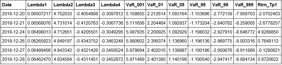
For the next exercise we will set up an out-of-sample procedure where we use a rolling 2-year window to calibrate the GLD parameters, then we estimate 0.1%, 1%, 5%, 95%, 99%, 99.9% VaR for the next day, and finally we compare it to subsequent day’s return. Based on all the observations we would expect 5% and 95% VaR to be exceeded in approximately 5% of the sample.

First, let’s set up the data frame that will hold our results.

N <- length(returns_xts)
lookback <- 251*2
sample_end <- lookback:N
sample_start <- 1:length(sample_end)
alpha1 <- .95
alpha2 <- .99
alpha3 <- .999

output_df <- data.frame(Date = as.Date(rep(NA, N-lookback)),
                       Lambda1 = numeric(N-lookback),
                       Lambda2 = numeric(N-lookback),
                       Lambda3 = numeric(N-lookback),
                       Lambda4 = numeric(N-lookback),
                       VaR_001 =  numeric(N-lookback),
                       VaR_01 =  numeric(N-lookback),
                       VaR_05 =  numeric(N-lookback),
                       VaR_95 =  numeric(N-lookback),
                       VaR_99 =  numeric(N-lookback),
                       VaR_999 =  numeric(N-lookback),
                       Rtrn_Tp1 =  numeric(N-lookback),
                       stringsAsFactors = FALSE)

Below is the main loop for the backtest. Please note that here I specify VaR 95 at the 5th percentile of returns because it is typical in finance to think of VaR in terms of losses. When one discusses 95% VaR it is the 5th percentile of the distribution that we are interested in. In the loop I use (1-alpha) as an argument to the quantile function.

# Main Loop
for (ii in 1:(N-lookback)){
    subset_sample <- coredata(returns_xts[sample_start[ii]:sample_end[ii],]) # extract the window
    my_gld_fit <- fun.RMFMKL.ml(data = subset_sample)  # calibrate parameters
    my_VaR <- qgl(c(c(alpha3, alpha2, alpha1), 1- c(alpha1, alpha2, alpha3)), lambda1 = my_gld_fit)  # calculate VaR
    
    # extract results
    output_df[ii, 'Date'] <- index(returns_xts[sample_end[ii]]) 
    output_df[ii, c(2,3,4,5)] <- my_gld_fit
    output_df[ii, c(6,7,8,9,10,11)] <- my_VaR
    output_df[ii, 'Rtrn_Tp1'] <- returns_xts[sample_end[ii]+1,1]
}

tail(output_df)

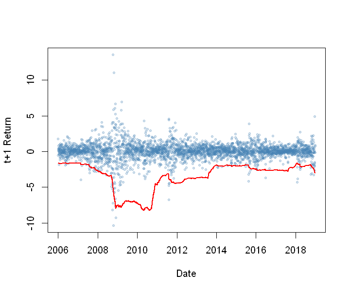
As a very quick check we simply count the number of times the observed t+1 return exceeded the estimated VaR. You can see that the fitted distribution does a decent job of matching our expectations. 5% VaR was exceeded 5.25% of the time. 95% VaR was exceeded 5.78% of the time.

round(sum(output_df[,'Rtrn_Tp1'] > output_df[,'VaR_001'])/length(returns_xts)*100,2)
round(sum(output_df[,'Rtrn_Tp1'] > output_df[,'VaR_01'])/length(returns_xts)*100,2)
round(sum(output_df[,'Rtrn_Tp1'] > output_df[,'VaR_05'])/length(returns_xts)*100,2)

round(sum(output_df[,'Rtrn_Tp1'] < output_df[,'VaR_95'])/length(returns_xts)*100,2)
round(sum(output_df[,'Rtrn_Tp1'] < output_df[,'VaR_99'])/length(returns_xts)*100,2)
round(sum(output_df[,'Rtrn_Tp1'] < output_df[,'VaR_999'])/length(returns_xts)*100,2)

0.21
1.35
5.25
5.78
1.38
0.11

Below I plotted daily returns and the 99% VaR as a red line.

plot(output_df[,'Date'], 
     output_df[,'Rtrn_Tp1'], 
     cex = .5, 
     pch = 19, 
     col = rgb(red = .275, green = .51, blue = .706, alpha =.25),
     ylab = 't+1 Return',
     xlab = 'Date')

lines(output_df[,'Date'], output_df[,'VaR_99'], col = 'red', lwd = 2)

This was a quick guide on how to implement a useful flexible distribution to model asset returns. In future posts I will introduce and explore other flexible distributions. Stay tuned.

Useful Resources:
1) Corlu, Canan G., and Alper Corlu. “Modelling Exchange Rate Returns: Which Flexible Distribution to Use?” Quantitative Finance, vol. 15, no. 11, 2014, pp. 1851–1864., doi:10.1080/14697688.2014.942231. Link

2) Corlu, Canan Gunes, et al. “Empirical Distributions of Stock Returns: A Comparison.” SSRN Electronic Journal, 2015, doi:10.2139/ssrn.2622672. Link