The previous two posts have dealt with hard and soft margin SVM.  In both cases our model used a linear (hyperplane) decision boundary.  The only difference between the two is that the soft margin classifier does not split the two classes perfectly because the data is not linearly separable.  We still used a hyperplane but made an allowance for violations of the margin that we control with the cost parameter.  Today we will continue looking at data that is not linearly separable but this time using a soft margin won’t help.

Let’s begin by looking at an example where we have a single feature in one dimension.  Positive class in blue cannot be linearly separated from the negative class in red.  You can clearly see that if we use a hard margin svm then our algorithm will not converge since the data is not linearly separable.  If we were to use the soft margin classifier we would be able to calibrate the model but the model performance will be terrible.

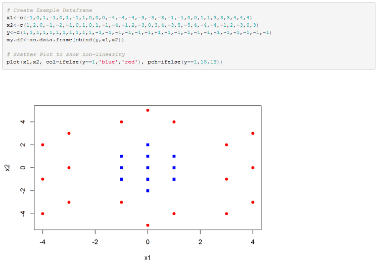
Below is another example, but this time in 2D.  Any attempts to use a linear decision boundary will fail miserably.

Feature Engineering:

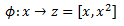
For example, in the first problem presented we can change our SVM decision boundary from wx+b=0, where w and x are 1D each, to a hyperplane wz+b=0 using new feature vector z=[x,x*x].

If we plot the new feature space we can clearly see that the classes are now linearly separable.

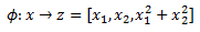
For the second example that we have we can again increase the dimension of our feature space and see if we can linearly separate the data.  So we change our model from wx+b=0 where x=[x1,x2]  to wz+b=0 where z=[x1,x2,x1^2+x2^2].  Plotting the classes in the new 3D feature space we can see that we can indeed separate the classes with a hyperplane.

It is standard to denote feature mapping with the Greek letter Phi.  For the first example we have:

For our second example we would write:

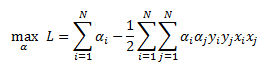
Recall that for our soft margin classifier we derived the dual optimization as:

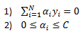
Subject to below two constraints:

So now that we decided to use our feature mapping function to increase the dimension of our feature space we can insert these functions into the SVM optimization function.  We get:

Next lets implement our SVM classifier just as we did in my previous posts to see if we can find a separating hyperplane in the higher dimension.

Below is my R implementation.  I first create the data and plot it.

Next we explicitly add a new feature to our data frame to increase the dimension of our feature space.

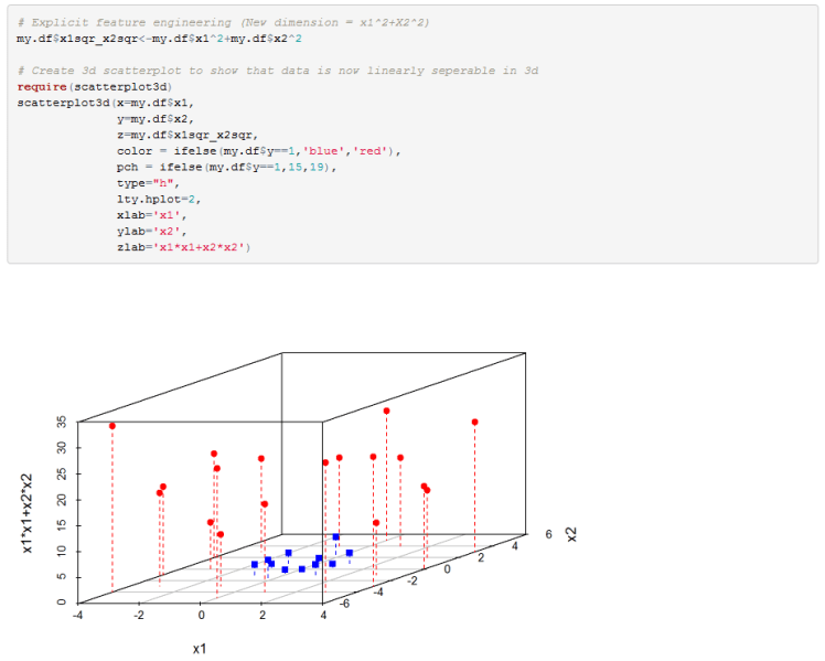
Here our Phi function would be defined as:

You can see from the 3D scatterplot that the two classes are linearly separable so let’s fit SVM to this data frame and compute our w and b coefficients.

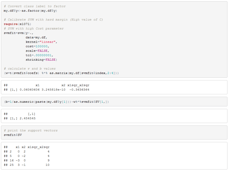
We can see that there are 4 support vectors.

I also set this problem up in excel and solved it using Solver. The workbook link is provided later in the post.  The relevant tab is ExplicitFeatureMapping.

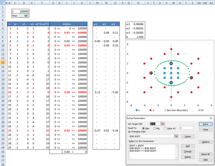
You can see that our results match R closely.  The difference is due to convergence criteria in R and excel.  The interesting thing I want you to note is that after solving our problem in the higher dimension we end up with the following decision boundary:

Plugging into our decision boundary equation

We get:

The key thing to note is that while we solved for a hyperplane in the higher dimension z we ended up with a non-linear decision boundary in our original feature space x.  You can see a plot of the decision boundary in the excel file.  The support vectors are highlighted in the plot.  While in this case the support vectors are close to our decision boundary they need not be when we are looking at our feature space x.  They could have been further away and not make much intuitive sense to us because they were solved for in feature space z not x.

To recap so far, we mapped our features to a higher dimension because our classes were not linearly separable.  We then searched for a linear classifier in the new feature space.  Once we find the separating hyperplane we plot it as a decision boundary in our original feature space and end up having a non-linear classifier.

Up to this point, if you have gone through all my posts on SVM, we have a method to find a large margin classifier for linear and non-linear data.  Furthermore, we have a way to allow for some violations of our margin via a tuning cost parameter.  It appears as though we have the tools to handle most practical classification problems.

Now for the bad news, there are two potential problems when we go into higher dimension feature space.  The first one is that when we increase the dimension of our features we run the risk of over fitting the model.  This is actually not a problem because we are using a model that tries to find the largest margin which controls for over fitting.  If we use cross-validation to select our tuning parameters we should end up with a model that generalizes well.  The second problem is more serious, it is that the dimensionality of the problem explodes quickly.  Suppose we have feature x1 and x2 and we wish to perform a 2-degree polynomial expansion of our features.  This means we would have the following:

This is very manageable but now think about what would happen in an image classification problem where we might be working with a 18×18 pixel image.  That gives us 324 features (one for each pixel).  If we decide that we need a non-linear SVM implementation and wanted to perform polynomial feature expansion we can see that the dimension of the feature space begins to be very large.

Kernel Trick:

There is a very cool trick to handle the problem stated above.  Notice that our data enters the algorithm only as a dot-product (highlighted in red).

What if we had a function that takes the original data and its output was dot product of the expanded features?  This will make things a lot more manageable from a computational point of view.   What I am saying is instead of explicitly mapping our features x into higher dimension z using phi and then taking the dot-product (like we did in previous example) lets use some function K(,) that takes our features x as input and returns the dot-product of z.  We can write this as:

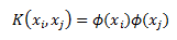
K is called a kernel and it has to satisfy some technical conditions.  In the useful resources section I link to Mercer’s condition wikipedia entry for those who are interested.

Some of the most popular kernels are:

In the above, gamma, b, d, and sigma are tuning parameters.

Once we settle on a kernel we no longer need to explicitly map our features to higher dimension using Phi.  Instead we plug our features x into our kernel and the output is the dot-product of the higher dimensional z space.  I should mention that we don’t need to know what z space is.  In case of radial basis kernel the space has infinite dimension!

So with our chosen kernel our algorithm becomes:

The constraints remain the same.

Rewriting in matrix notation we have:

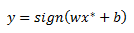
Once we find our alphas we need to recover our vector w and coefficient b so we can classify new data points.

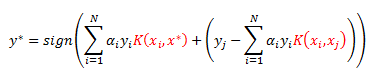
Our classification rule for some point x star is given as:

From my previous post we derived w as a function of alphas from KKT conditions that must hold at the solution of our optimization problem.

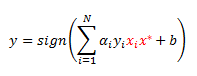
Let’s plug this into our classification rule to get:

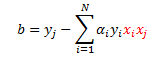
Now let’s remember the formula for coefficient b.  Recall from my previous post that b can be calculated from a support vector (point with a positive alpha) that has a slack variable of zero, call it point j:

Once again, plug in our definition of w:

Notice I have been highlighting the dot-products.  We again use our kernel to get the following decision boundary:

R Implementation:

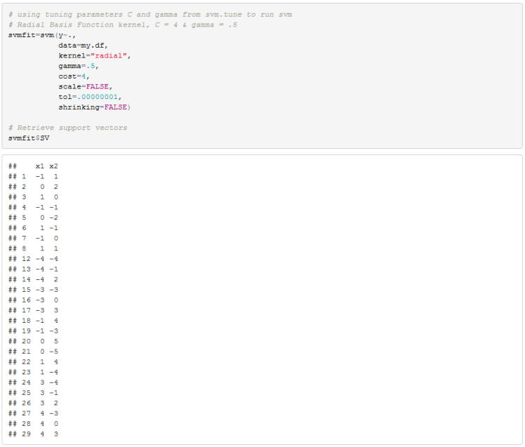
I first recreated our dataset and performed a search for optimal gamma and cost parameters using a radial basis function kernel.

We can now run the SVM algorithm with C equal to 4 and gamma equal to .5.  We will later compare these results to our excel implementation.

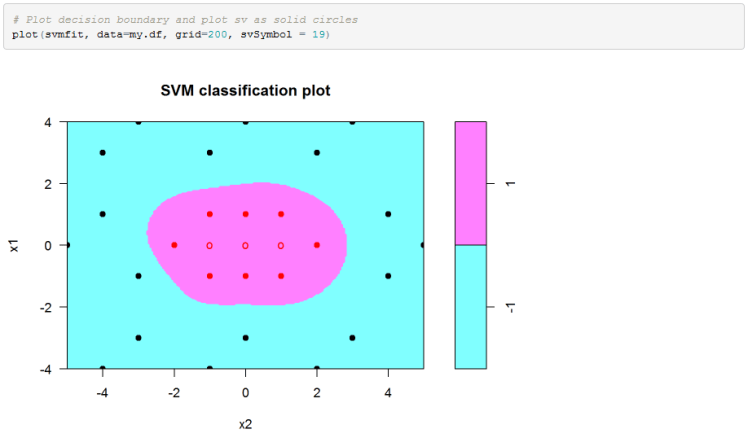
Finally we can plot the decision boundary in the original feature space.  Please note that for some reason e1071 package in R reverses the axis in the SVM plot.

Excel Implementation:

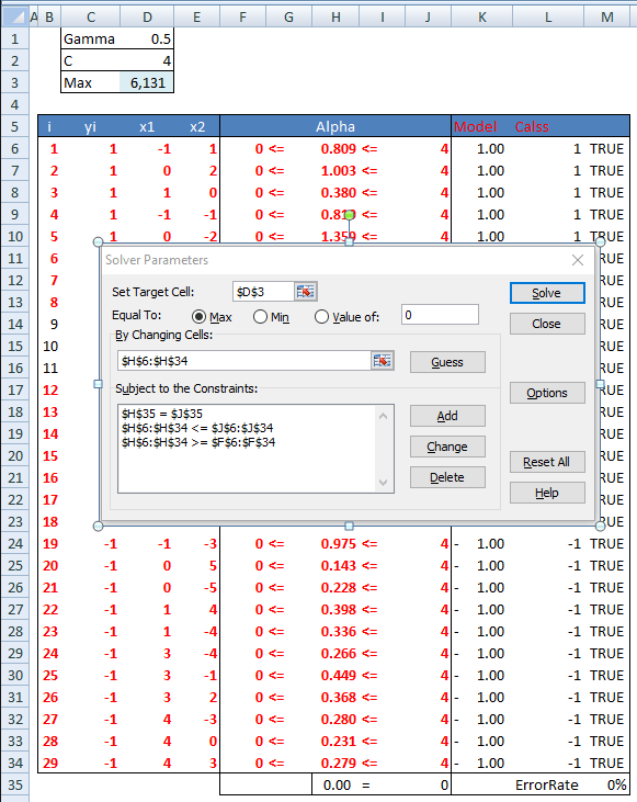
In the workbook we have a tab with ImplicitFeatureMappig(Kernel) tab that implements this model in excel.  We first calculate kernel function values using array formulas in range C74:AE102.  Then we calculate the quadratic coefficients matrix in range C41:AE69. The objective function value is in cell D3.  The constraints are in column H.  Then we can run Solver to get the alphas.  Coefficient b is calculated in cell R5 using our second support vector.  Our results are very close to R’s output. svm_kernel_calcs_example

Hope you enjoyed.

Some Useful Resources:

• Michael Jordan’s “The Kernel Trick” in Advanced Topics in Learning & Decision Making course notes http://people.eecs.berkeley.edu/~jordan/courses/281B-spring04/lectures/lec3.pdf
• Andrew Ng notes http://cs229.stanford.edu/notes/cs229-notes3.pdf
• Lecture 15 on Kernel Methods from Yaser Abu-Mostafa at Caltech https://work.caltech.edu/telecourse.html
• Barnabas Poczos slides on Kernel Methods http://www.cs.cmu.edu/~aarti/Class/10701_Spring14/slides/kernel_methods.pdf
• R e1071 package description https://cran.r-project.org/web/packages/e1071/e1071.pdf
• Wikipedia page for Mercer’s condition that kernels need to satisfy https://en.wikipedia.org/wiki/Mercer%27s_theorem#Mercer.27s_condition.