Quantile Regression

In this post, I would like to quickly introduce what I believe to be an underutilized modelling technique that belongs in most analysts’ toolkit: the quantile regression model. As I am discussing some of the main points, I will be working with R’s quantreg package that is maintained by the inventor of quantile regression. See link here for more details.

To highlight the benefits of building quantile regression models, I will contrast it with the ubiquitous linear regression model.

Regression models are used to study a relationship between a dependent (target) variable and some set of independent (explanatory) variables. We use explanatory variables to estimate what the mean/expected value of the target variables is conditioned on the observed explanatory variables. Here is the usual expression:

$y_{t}=E\left[Y_{t}\right]+\epsilon_{t}=\alpha+\beta x_{t}+\epsilon_{t}$

Here $y_{t}$ is the average value $E\left[Y_{t}\right]$ plus some noise $\epsilon_{t}$ . The expected value is equal to $\alpha + \beta x_{t}$ . Notice that we are studying the central moment (the mean) of the dependent variable based on some explanatory variables. But we are often interested in much more than just the expected value. This is not an issue if the error term is normally distributed, has a mean of zero, and a constant variance $\sigma^{2}$ . In that case, $E\left[Y_{t}\right] + \epsilon_{t}$ is normally distributed and we know everything about the distribution. We only need the mean and the variance to describe the data in case of a normal distribution. But as we all know, normality assumption is almost always violated when dealing with financial or economic data.

So what are we supposed to do when mean and variance are not enough. We need to get other information about the distribution. Higher order moments are important, e.g. skewness and kurtosis. Another way to describe the data is via its quantiles. For example, instead of the mean, we can use the median as the measure of central tendency. This often makes sense for skewed distributions. We can also examine interquartile range by looking at the difference between 75th and 25th percentile of the distribution.

This idea gave rise to the quantile regression model. Instead of modelling the mean/expected value of the target variable, let’s instead model some quantile of the data conditional on some explanatory variable. When we do that, we can estimate a set of models for some specified set of quantiles. Conditioning on explanatory variables, we will have a much more granular view of the distribution of the target variable. We can observe changes in the distribution (shape shift) at different values of the explanatory variable. This is incredibly useful when answering specific questions.

Let’s write an equation to solidify the concept. We have:

$y_{t}=Q^{p}\left[Y_{t}\right]+\varepsilon_{t}^{p}=\alpha^{p}+\beta^{p} x_{t}+\varepsilon_{t}^{p}$

Here $Q^{p}\left[Y_{t}\right]$ is the $p^{th}$ quantile of the variable $Y_{t}$ . Obviously, 0 < p < 1. So, for example, if we are modelling the median (50th percentile) then that would be our definition of $y_{t}$ , and we would have some set of estimated parameters ( $\alpha^{median}, \beta^{median}$ ). If we are also interested in the 10th percentile, then we would estimate another model where $y_{t}$ is now the 10th percentile of the target variable. We will obviously have another set of estimated parameters ( $\alpha^{10percentile}, \beta^{10percentile}$ ).

This is incredibly useful – we can analyze the impact of the explanatory variables on the full distribution of the target variable with fewer assumptions than in OLS.

Let’s use the example from quantreg vignette. See link here for more details.

require(quantreg)

data(engel)
attach(engel)
plot(income,foodexp,cex=.25,type="n",xlab="Household Income", ylab="Food Expenditure")
points(income,foodexp,cex=.5,col="blue")
abline(rq(foodexp~income,tau=.5),col="blue")
abline(lm(foodexp~income),lty=2,col="red") #the dreaded ols line
taus <- c(.05,.1,.25,.75,.90,.95)
for( i in 1:length(taus)){
    abline(rq(foodexp~income,tau=taus[i]),col="gray")
}

Here, we model household food expenditure as a function of income. The red line is the OLS regression line, the blue line is the median regression line, and the grey lines are the 5th, 10th, 25th, 75th, 90th, and 95th quantile lines. Notice that the quantiles capture shape shift of the distribution. At low income levels, the spread in the distribution is tight. For large incomes, household food expenditures have a very wide distribution. Also, notice that the difference is small between the 95th and 90th quantile, but the difference is big between the 5th and 10th quantile. There is so much more information here than usual OLS regression model.

It is also important to mention that the results are much more robust than the usual regression model. This is because we are modelling quantiles which are much less sensitive to outliers if they remain on the correct side of the quantile. This simply means that if, for example, we have a very large negative observed value, our estimate of ( $\alpha^{median}, \beta^{median}$ ) does not change because the median of the distribution does not register the magnitude of the values, just their ranking.

One final comment before we start to get our hands dirty. Please note that in the usual regression model, we fit the parameters so that the error term $\epsilon_{t}$ has a mean of zero. Since in quantile regression model we define $y_{t}$ as the conditional quantile plus the error term, $Q^{p}\left[Y_{t}\right]+\varepsilon_{t}^{p}$ , the value $Q^{p}\left[Y_{t}\right]$ conditional on $x_{t}$ is constant and equal to $\alpha^{p}+\beta^{p} x_{t}$ . This means the error term in the quantile regression $\varepsilon_{t}^{p}$ is related to the ordinary regression error term as: $\varepsilon_{t}^{p} = Q^{p}\left[\epsilon_{t}\right]$ . i.e. in quantile regression, we require that the $p^{th}$ quantile of the error term be zero.

I don’t want to do a deep dive of how the parameters are estimated. This is an interesting topic and more info is available in the references I provide at the end of the post. Let me just make two points. First, there is no closed form solution. We need our software to perform numerical routines and hope they converge to an optimal solution. Luckily this issue has been studied for a long time and reliable numerical routines have been implemented for us. Second, though it is not obvious, the solutions are derived by minimizing below function.

$\min _{\alpha, \beta} \sum_{t=1}^{T}\left(p-\mathbf{1}_{y_{t} \leq \alpha+\beta x_{t}}\right)\left(y_{t}-\left(\alpha+\beta x_{t}\right)\right)$ ,

where

$\mathbf{1}_{y_{t} \leq \alpha+\beta x_{t}}=\left\{\begin{array}{ll}{1} & {\text { if } y_{t} \leq \alpha+\beta x_{t}} \\ {0} & {\text { otherwise }}\end{array}\right.$

The idea is very similar to OLS where we estimate our parameters by minimizing some loss function. In the case of OLS we minimize sum of squared errors. In quantile regression, our cost function is asymmetric and depends on what quantile p we are estimating.

Now, time to get our hands dirty. Let’s work our way through an example that is very relevant in macro land these days. The Fed and markets are worried about the uncertainty about growth and market is pricing in insurance cuts from the Fed. Everyone seems to be in universal agreement that downside risks have increased this year and that it warrants a policy response from the Fed. So what we want to do here is estimate future GDP distribution conditioned on some economic variables and see if we can quantify the increase in uncertainty. There are some interesting papers that have been published by Fed researchers that tackle this problem directly. I provide the link at the end of the post, but click here if you want to have a look before proceeding.

The idea is that we can do the following:

Model the quantile of 1-year forward GDP as a function of current GDP and a broad measure of financial conditions. In the paper they use average GDP prints from current quarter out to 4 quarters ahead. I will instead model actual GDP print 4 quarters ahead. Also, the financials conditions index that we are using is released on a weekly basis. I use a 3-month average as an input into the model. More info about the index can be found here.
After estimating the quantiles, the authors fit a skewed Student-t distribution to get the full distribution. The authors solved for the 4 parameters of the distribution directly to match the 5th, 25th, 75th, and 95th quantile. In this post, we will estimate more quantile regression models and fit a Student-t by minimizing sum of squared residuals.
Once we have a full fitted distribution, we can calculate expected shortfall for GDP. We can then monitor the evolution of GDP tails risk conditional on current growth and financial conditions.

If you want to follow along, I have the data at the end of the blog. This data can be found online (publicly available) but I attached here for your convenience.

First, let’s fit the models for 5th, 10th, 15th, 25th, 35th, 50th, 65th, 75th, 85th, 90th, and 95th quantiles.

# fit quantile regression for 11 quantiles
my_taus <- c(.05, .10, .15, .25, .35, .50, .65, .75, .85, .90, .95)
my_qr_fit <- rq(GDP_Tp4 ~ GDP + NFCI, 
                tau = my_taus, 
                data = in_sample_data) # in_sampe_data is my raw data file

We can then look at the statistical significance of the estimated parameters. Please note that we need to run a bootstrap method to estimate the coefficients’ standard errors. Basically, we resample all the data with replacement many times (200 is the default). We estimate our coefficients using each sample. After we have bootstrapped estimates, we can calculate their standard errors

# check for statistical significance via bootstrap
my_summary <- summary(my_qr_fit, se = 'boot')
my_summary

Call: rq(formula = GDP_Tp4 ~ GDP + NFCI, tau = my_taus, data = in_sample_data)
 tau: [1] 0.05
 Coefficients:
             Value    Std. Error t value  Pr(>|t|)
 (Intercept) -2.34612  0.76494   -3.06705  0.00271
 GDP          0.32266  0.29841    1.08126  0.28190
 NFCI        -4.34642  0.81119   -5.35805  0.00000
 Call: rq(formula = GDP_Tp4 ~ GDP + NFCI, tau = my_taus, data = in_sample_data)
 tau: [1] 0.1
 Coefficients:
             Value    Std. Error t value  Pr(>|t|)
 (Intercept) -1.06657  0.80660   -1.32230  0.18876
 GDP         -0.03196  0.30036   -0.10642  0.91544
 NFCI        -4.45513  0.77950   -5.71534  0.00000
 Call: rq(formula = GDP_Tp4 ~ GDP + NFCI, tau = my_taus, data = in_sample_data)
 tau: [1] 0.15
 Coefficients:
             Value    Std. Error t value  Pr(>|t|)
 (Intercept) -0.77808  0.82633   -0.94161  0.34842
 GDP          0.03824  0.23594    0.16206  0.87155
 NFCI        -3.95458  0.89826   -4.40250  0.00002
 Call: rq(formula = GDP_Tp4 ~ GDP + NFCI, tau = my_taus, data = in_sample_data)
 tau: [1] 0.25
 Coefficients:
             Value    Std. Error t value  Pr(>|t|)
 (Intercept)  0.31032  0.80157    0.38713  0.69939
 GDP          0.02821  0.15774    0.17882  0.85840
 NFCI        -3.12373  1.13956   -2.74117  0.00713
 Call: rq(formula = GDP_Tp4 ~ GDP + NFCI, tau = my_taus, data = in_sample_data)
 tau: [1] 0.35
 Coefficients:
             Value    Std. Error t value  Pr(>|t|)
 (Intercept)  0.76880  0.75029    1.02468  0.30772
 GDP         -0.01704  0.15815   -0.10772  0.91441
 NFCI        -2.75392  0.90770   -3.03393  0.00300
 Call: rq(formula = GDP_Tp4 ~ GDP + NFCI, tau = my_taus, data = in_sample_data)
 tau: [1] 0.5
 Coefficients:
             Value    Std. Error t value  Pr(>|t|)
 (Intercept)  1.64539  0.65757    2.50221  0.01379
 GDP          0.02938  0.18618    0.15782  0.87488
 NFCI        -1.63139  0.84303   -1.93514  0.05549
 Call: rq(formula = GDP_Tp4 ~ GDP + NFCI, tau = my_taus, data = in_sample_data)
 tau: [1] 0.65
 Coefficients:
             Value    Std. Error t value  Pr(>|t|)
 (Intercept)  2.47940  0.56079    4.42127  0.00002
 GDP          0.09154  0.21980    0.41646  0.67787
 NFCI        -0.86369  0.82591   -1.04574  0.29793
 Call: rq(formula = GDP_Tp4 ~ GDP + NFCI, tau = my_taus, data = in_sample_data)
 tau: [1] 0.75
 Coefficients:
             Value    Std. Error t value  Pr(>|t|)
 (Intercept)  3.09624  0.39588    7.82120  0.00000
 GDP          0.14126  0.16218    0.87102  0.38561
 NFCI        -0.60402  0.62649   -0.96413  0.33706
 Call: rq(formula = GDP_Tp4 ~ GDP + NFCI, tau = my_taus, data = in_sample_data)
 tau: [1] 0.85
 Coefficients:
             Value    Std. Error t value  Pr(>|t|)
 (Intercept)  3.44024  0.30096   11.43101  0.00000
 GDP          0.15078  0.10782    1.39837  0.16476
 NFCI        -0.57208  0.43038   -1.32925  0.18647
 Call: rq(formula = GDP_Tp4 ~ GDP + NFCI, tau = my_taus, data = in_sample_data)
 tau: [1] 0.9
 Coefficients:
             Value    Std. Error t value  Pr(>|t|)
 (Intercept)  3.73520  0.24207   15.43012  0.00000
 GDP          0.22777  0.06743    3.37786  0.00101
 NFCI        -0.04564  0.41388   -0.11028  0.91238
 Call: rq(formula = GDP_Tp4 ~ GDP + NFCI, tau = my_taus, data = in_sample_data)
 tau: [1] 0.95
 Coefficients:
             Value    Std. Error t value  Pr(>|t|)
 (Intercept)  3.88112  0.16259   23.87047  0.00000
 GDP          0.22079  0.06693    3.29861  0.00130
 NFCI        -0.04759  0.39025   -0.12194  0.90317

There is a lot of output to digest. First, notice that for lower quantiles it is the financial conditions that are important, not current economic conditions. The alternative seems to be true for higher quantiles.

A much better way to view the output is via coefficient plots.

# coefficient plots
plot(my_summary)

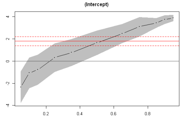
From these plots we can immediately see that for lower quantiles, financial conditions index coefficients and their confidence bands are significantly different from zero. This is not the case for GDP coefficients.

Now that we have the fitted models, let’s extract the estimated quantiles.

# extract fitted quantiles based on model
my_predict <- predict(my_qr_fit)

We now need to be able to calibrate a Skewed Student-t (SST) distribution to these quantiles. To do this, we can set up a minimization routine. First, we will write an objective function that takes as arguments the 4 parameters of the SST distribution, the quantiles we are targeting, and the values of those quantiles. The function will return the sum of squared of the difference.

# objective function to fit
my_obj_fun <- function(my_dp, taus, target_quantile){
    # dp:                 trial a vector of length 4, elements represent location, scale, skew, and degrees of freedom
    # taus:               percentiles we are looking at (length of taus should match target_quantile)
    # target_quantile:    the empirical/model percentiles that we want GLD to match
    
    fitted_quantiles <- sn::qst(taus, dp = my_dp)
    not_inf <- !is.infinite(fitted_quantiles)
    result <- sqrt(sum((target_quantile[not_inf] - fitted_quantiles[not_inf])^2))*100
    return(result)
}

We will then write a function that uses R’s optimization routine to minimize our objective function:

# minimization routine
my_solver <- function(target_quantile, init_values, taus){
    result <- optim(init_values, 
                 my_obj_fun, 
                 taus = taus,  
                 target_quantile = target_quantile, 
                 method = 'Nelder-Mead', 
                 control = list(maxit = 100, abstol = .000001))$par
    
    return(result)
}

Now we will first fit an SST distribution to all our GDP observations to get a set of good starting values to feed into our minimization routine.

require(sn)
SST_Fit <- sn::st.mple(y=in_sample_data[,'GDP'])
initial_values <- SST_Fit$dp

And let’s plot the fitted distribution along with the histogram of the actual distribution of quarterly GDP prints.

hist(in_sample_data[,'GDP'],
 col='peachpuff', 
 border='black',
 prob = TRUE, # show densities instead of frequencies
 xlab = 'GDP',
 xlim=c(-5,6),
 breaks=20,
 main = '')

lines(x = seq(-5,6, by = .05), 
      y = dst(seq(-5,6, by = .05), dp=initial_values),
 lwd = 3, # thickness of line
 col = 'steelblue')

Let’s try this now to calibrate a SST distribution to the first set of fitted quantiles from our regression model.

# try solver on one observation
test_param <- my_solver(target_quantile = my_predict[1,], 
                        initial_values, 
                        taus = my_taus)

And let’s see quantiles from our calibrated distribution based on the fitted parameters.

sn::qst(my_taus, dp = test_param)

-1.82167377991434  -0.897478033842928  -0.317201996236203
0.488771386216558  1.09817828817344  1.87586807146716  2.62893251134214
3.18728127939248  3.88910109003964  4.3725835716495  5.11220664005463

my_predict[1,]

-1.08828972132954  -1.1917950846466  -0.629463584621562
0.41992958066738  0.702009508800799  1.75977359546504  2.83628037426853
3.64709619438839  4.02819298775264  4.62350035122945  4.74217692823193

And one more time for another set of estimated quantiles via quantile regression:

# try solver on one observation
test_param <- my_solver(target_quantile = my_predict[10,], 
                        initial_values, 
                        taus = my_taus)

sn::qst(my_taus, dp = test_param)

0.361081016667099  0.976569681870633  1.35985579676273  1.88170447048113
2.26245622070612  2.72305723000699  3.13679995549024  3.42278780682794
3.75976486690277  3.97940161356939  4.29917698946775

my_predict[10,]

0.297148107584487  1.20757328502942  1.32048689850673  1.96558089844999
2.17781950506346  2.52744469760649  3.03755265206431  3.57928464901055
3.91811899382793  4.03221608883146  4.17076043833115

Now, let’s loop through all our observations and fit an SST distribution at each point in time.

fitted_sst_params <- t(apply(my_predict, 
                             MARGIN = 1, 
                             FUN = my_solver, 
                             init_values = initial_values, 
                             taus = my_taus))

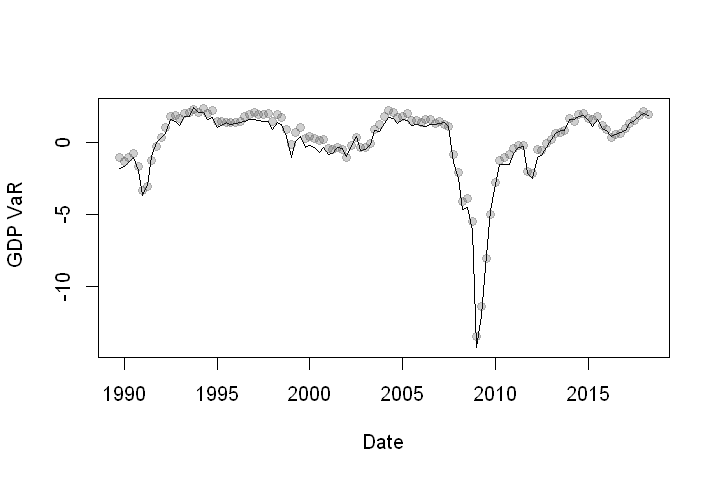
We can now compute GDP at 5% VaR. This is basically the 5th quantile that can be calculated as below.

N <- nrow(my_predict)
GDP_VAR <- rep(NA, N)
for (ii in 1:N){
    GDP_VAR[ii] <- sn::qst(p = .05, dp = fitted_sst_params[ii,])
}

Now, let’s plot a time series of GDP at 5% VaR. In our plot, the 5th quantile from the fitted SST is plotted as a line. I included grey dots that come straight from the fitted quantile regression for reference also. Any difference between the two is simply a function of our fitting error earlier.

plot(in_sample_data[,'Date'], 
     GDP_VAR, 
     type = 'l', 
     xlab='Date', 
     ylab=' GDP VaR')

points(in_sample_data[,'Date'],my_predict[,1], pch = 19, col = rgb(.25,.25,.25,.25))

Next, calculate the expected shortfall.

# function for Expected Shortfall (Conditional VAR) (numerically integrate from 0 to alpha)
SST_ES <- function(params, alpha = .05){
    result <- 1/(alpha) * integrate(sn::qst, lower = .00001, upper = alpha, stop.on.error = TURE, dp = params)$value
    return(result)
}

# calculate ES for each quarter
GDP_ES <- apply(fitted_sst_params, MARGIN = 1, FUN = SST_ES)

# Plot ES on a rolling-base
plot(in_sample_data[,'Date'], GDP_ES, type = 'l', xlab='Date', ylab=' GDP ES', ylim = c(-20,5))

Notice that we get close to the results of Adrian et al. (2019).

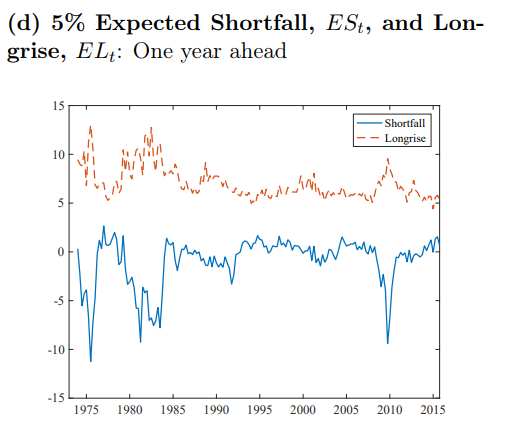
Note that our results are not identical because we have defined the problem slightly differently. Here we are modelling the distribution of the quarterly GDP print four quarters in the future, while Adrian et al. (2019) are modelling the distribution of the average of four furture quarterly GDP readings.

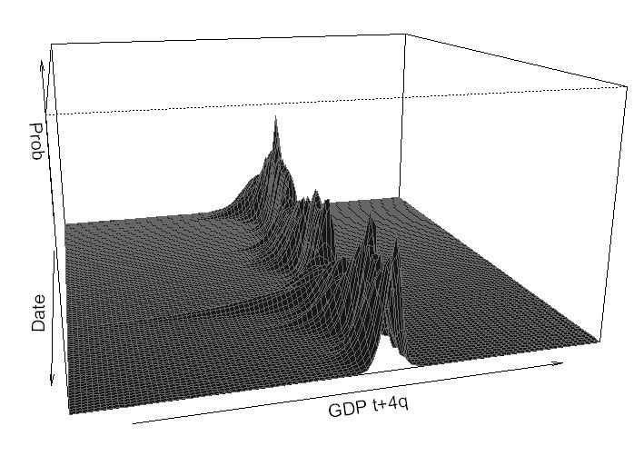
Now, I want to demonstrate a 3-D plot of how GDP distribution evolves over time according to our model.

# data for plot
GDP_Plot <- seq(-25, 25, by = .5)
Prob_Plot <- matrix(NA, nrow = length(in_sample_data[,'Date']), ncol = length(GDP_Plot))

for (ii in 1:length(in_sample_data[,'Date'])){
    Prob_Plot[ii,] <- sn::dst(GDP_Plot, dp = fitted_sst_params[ii,])
}


require(grDevices)
persp(x = 1:115,
      y = GDP_Plot,
      z = Prob_Plot,
      xlab = 'Date',
      ylab = 'GDP t+4q',
      zlab = 'Prob',
      xlim = c(1,115),
      ylim = c(-25,25),
      zlim = c(0,1.1),
      theta = 75,
      phi = 15,
      col = 'grey9',
      #col =  color[facetcol],
      border='grey40',
      expand = 0.5)

Finally, we can also generate scenarios using our model. We first create a data frame to hold our scenarios, then feed them into our quantile regression to get the estimated quantiles, and finally, we fit the skewed student t distribution to the quantiles.

# scenario data
scenario_data <- data.frame(GDP = c(-1.0, 1.5, 3.0),
                            NFCI = c(1.5, 0.0, -.50),
                            stringsAsFactors = FALSE)

#fitted quantiles based on model
scenario_quantiles <- predict(my_qr_fit, newdata = scenario_data)

#skewed student t parameters for scenarios
scenario_sst_params <- t(apply(scenario_quantiles, 
                             MARGIN = 1, 
                             FUN = my_solver, 
                             init_values = initial_values, 
                             taus = my_taus))

Now we can plot the distributions.

# plot 
gdp_grid <- seq(-20,15, by = .25)
plot(gdp_grid, sn::dst(gdp_grid, dp = scenario_sst_params[1,]), type= 'l', lty = 1,
     xlab='Prob', ylab= 'GDP t+4q',  ylim=c(0, .4))
polygon(gdp_grid, sn::dst(gdp_grid, dp = scenario_sst_params[1,]),col=rgb(.5, .95, .75, .15))

lines(gdp_grid, sn::dst(gdp_grid, dp = scenario_sst_params[2,]))
polygon(gdp_grid, sn::dst(gdp_grid, dp = scenario_sst_params[2,]),col=rgb(.7, .1, .4, 0.15))


lines(gdp_grid, sn::dst(gdp_grid, dp = scenario_sst_params[3,]))
polygon(gdp_grid, sn::dst(gdp_grid, dp = scenario_sst_params[3,]),col=rgb(1, 0, 1, .15))

legend("topleft", legend=c('Scn1', 'Scn2', 'Scn3'),
       col=c('seagreen3', 'violetred4', 'violet'), lty = 1, inset=.02, cex = .6, y.intersp=2.5)

I hope I convinced you that quantile regression is a powerful tool. It can be very effective for capturing conditional distribution of some variable of interest. Good luck!

Resources

Adrian, Tobias, et al. Vulnerable Growth – FEDERAL RESERVE BANK of NEW YORK, www.newyorkfed.org/research/staff_reports/sr794
Loria, et al. “Assessing Macroeconomic Tail Risk.” SSRN, 19 Apr. 2019, papers.ssrn.com/sol3/papers.cfm?abstract_id=3375006
FINANCIAL CONDITIONS AND GROWTH AT RISK – IMF. www.imf.org/en/Publications/GFSR/Issues/2017/09/27/~/media/Files/Publications/GFSR/2017/October/chapter-3/Documents/c3.ashx?la=en
“National Financial Conditions Index (NFCI).” National Financial Conditions Index (NFCI) – Federal Reserve Bank of Chicago, www.chicagofed.org/publications/nfci/index
Koenker, Roger. “Quantile Regression [R Package Quantreg Version 5.41].” The Comprehensive R Archive Network, Comprehensive R Archive Network (CRAN), cran.r-project.org/web/packages/quantreg/index.html

# data for the model
 in_sample_data <- read.csv(header = TRUE, 
                             text = 'Date, GDP, NFCI, GDP_Tp4 
                                     30-09-1989, 3.9, 0.000127008, 1.7
                                     31-12-1989, 2.7, -0.036629133, 0.6
                                     31-03-1990, 2.8, -0.090870083, -1
                                     30-06-1990, 2.4, -0.182160633, -0.5
                                     30-09-1990, 1.7, -0.02811965, -0.1
                                     31-12-1990, 0.6, 0.277148608, 1.2
                                     31-03-1991, -1, 0.091021233, 2.9
                                     30-06-1991, -0.5, -0.288714925, 3.2
                                     30-09-1991, -0.1, -0.480414508, 3.7
                                     31-12-1991, 1.2, -0.51906455, 4.4
                                     31-03-1992, 2.9, -0.564142033, 3.3
                                     30-06-1992, 3.2, -0.718176483, 2.8
                                     30-09-1992, 3.7, -0.685154442, 2.3
                                     31-12-1992, 4.4, -0.59803585, 2.6
                                     31-03-1993, 3.3, -0.755371775, 3.4
                                     30-06-1993, 2.8, -0.799939058, 4.2
                                     30-09-1993, 2.3, -0.896682492, 4.3
                                     31-12-1993, 2.6, -0.824130317, 4.1
                                     31-03-1994, 3.4, -0.821335817, 3.5
                                     30-06-1994, 4.2, -0.685582642, 2.4
                                     30-09-1994, 4.3, -0.727856025, 2.7
                                     31-12-1994, 4.1, -0.567921583, 2.2
                                     31-03-1995, 3.5, -0.608324375, 2.6
                                     30-06-1995, 2.4, -0.671981133, 4
                                     30-09-1995, 2.7, -0.648721525, 4.1
                                     31-12-1995, 2.2, -0.696705942, 4.4
                                     31-03-1996, 2.6, -0.681872408, 4.3
                                     30-06-1996, 4, -0.649720717, 4.3
                                     30-09-1996, 4.1, -0.677856925, 4.7
                                     31-12-1996, 4.4, -0.692815608, 4.5
                                     31-03-1997, 4.3, -0.661724692, 4.9
                                     30-06-1997, 4.3, -0.656140467, 4.1
                                     30-09-1997, 4.7, -0.655591383, 4.1
                                     31-12-1997, 4.5, -0.532616742, 4.9
                                     31-03-1998, 4.9, -0.6195233, 4.8
                                     30-06-1998, 4.1, -0.621981908, 4.7
                                     30-09-1998, 4.1, -0.442741983, 4.7
                                     31-12-1998, 4.9, -0.136276067, 4.8
                                     31-03-1999, 4.8, -0.345186308, 4.2
                                     30-06-1999, 4.7, -0.429547225, 5.3
                                     30-09-1999, 4.7, -0.2570176, 4.1
                                     31-12-1999, 4.8, -0.277550325, 3
                                     31-03-2000, 4.2, -0.293507592, 2.3
                                     30-06-2000, 5.3, -0.176782192, 1.1
                                     30-09-2000, 4.1, -0.283548017, 0.5
                                     31-12-2000, 3, -0.220909875, 0.2
                                     31-03-2001, 2.3, -0.257047708, 1.3
                                     30-06-2001, 1.1, -0.3745106, 1.3
                                     30-09-2001, 0.5, -0.3794091, 2.2
                                     31-12-2001, 0.2, -0.275062117, 2.1
                                     31-03-2002, 1.3, -0.384926792, 1.8
                                     30-06-2002, 1.3, -0.518591775, 2
                                     30-09-2002, 2.2, -0.28980035, 3.3
                                     31-12-2002, 2.1, -0.305308933, 4.3
                                     31-03-2003, 1.8, -0.390609775, 4.3
                                     30-06-2003, 2, -0.592714233, 4.2
                                     30-09-2003, 3.3, -0.579556617, 3.4
                                     31-12-2003, 4.3, -0.636004083, 3.3
                                     31-03-2004, 4.3, -0.728082242, 3.9
                                     30-06-2004, 4.2, -0.70020205, 3.6
                                     30-09-2004, 3.4, -0.676979208, 3.5
                                     31-12-2004, 3.3, -0.708622083, 3.1
                                     31-03-2005, 3.9, -0.700670808, 3.4
                                     30-06-2005, 3.6, -0.618226142, 3.1
                                     30-09-2005, 3.5, -0.624520042, 2.4
                                     31-12-2005, 3.1, -0.621440575, 2.6
                                     31-03-2006, 3.4, -0.655807208, 1.5
                                     30-06-2006, 3.1, -0.665672808, 1.8
                                     30-09-2006, 2.4, -0.65326455, 2.2
                                     31-12-2006, 2.6, -0.684736175, 2
                                     31-03-2007, 1.5, -0.70984855, 1.1
                                     30-06-2007, 1.8, -0.659238383, 1.1
                                     30-09-2007, 2.2, -0.175482867, 0
                                     31-12-2007, 2, 0.095068958, -2.8
                                     31-03-2008, 1.1, 0.493424692, -3.3
                                     30-06-2008, 1.1, 0.439167758, -3.9
                                     30-09-2008, 0, 0.722941642, -3
                                     31-12-2008, -2.8, 2.342395083, 0.2
                                     31-03-2009, -3.3, 1.827469433, 1.7
                                     30-06-2009, -3.9, 1.027353242, 2.8
                                     30-09-2009, -3, 0.394184042, 3.2
                                     31-12-2009, 0.2, 0.118619033, 2.6
                                     31-03-2010, 1.7, -0.125451367, 1.9
                                     30-06-2010, 2.8, -0.095603975, 1.7
                                     30-09-2010, 3.2, -0.114889233, 0.9
                                     31-12-2010, 2.6, -0.25043795, 1.6
                                     31-03-2011, 1.9, -0.341584208, 2.7
                                     30-06-2011, 1.7, -0.358413492, 2.4
                                     30-09-2011, 0.9, -0.007418492, 2.5
                                     31-12-2011, 1.6, 0.081366008, 1.5
                                     31-03-2012, 2.7, -0.227845667, 1.6
                                     30-06-2012, 2.4, -0.232090867, 1.3
                                     30-09-2012, 2.5, -0.341464892, 1.9
                                     31-12-2012, 1.5, -0.480014042, 2.6
                                     31-03-2013, 1.6, -0.562598125, 1.5
                                     30-06-2013, 1.3, -0.605581217, 2.6
                                     30-09-2013, 1.9, -0.592675233, 3
                                     31-12-2013, 2.6, -0.717339183, 2.7
                                     31-03-2014, 1.5, -0.7624705, 3.8
                                     30-06-2014, 2.6, -0.790339467, 3.4
                                     30-09-2014, 3, -0.774638708, 2.4
                                     31-12-2014, 2.7, -0.71241615, 2
                                     31-03-2015, 3.8, -0.625803008, 1.6
                                     30-06-2015, 3.4, -0.698488767, 1.3
                                     30-09-2015, 2.4, -0.622464742, 1.5
                                     31-12-2015, 2, -0.600945333, 1.9
                                     31-03-2016, 1.6, -0.501130675, 1.9
                                     30-06-2016, 1.3, -0.561193167, 2.1
                                     30-09-2016, 1.5, -0.565286533, 2.3
                                     31-12-2016, 1.9, -0.625796542, 2.5
                                     31-03-2017, 1.9, -0.700084275, 2.6
                                     30-06-2017, 2.1, -0.738209208, 2.9
                                     30-09-2017, 2.3, -0.788917608, 3
                                     31-12-2017, 2.5, -0.83847425, 3
                                     31-03-2018, 2.6, -0.781312675, 3.2',
                             stringsAsFactors = FALSE)

2 thoughts on “Quantile Regression”

Pingback: Quantocracy's Daily Wrap for 07/15/2019 | Quantocracy
N_Cort says:

September 18, 2019 at 2:54 pm

Hi asmquant,

thanks a lot for your insights (I’ve been following this website since few years ago).
I m trying to make something similar with Chinese GDP with different features; while running the section

# try solver on one observation
test_param 3 & all(alpha * z > -5) & (tau == 0L)) “T.Owen” else “biv.nt.prob” :
missing value where TRUE/FALSE needed
Called from: psn(x, dp = dp0, …)

I guess it’s an unfeasible procedure for my specific analysis as the solver is finding some NAs in its routine.

Did you ever experienced something similar?

Many tks

LikeLike

Share this:

Related

2 thoughts on “Quantile Regression”

Leave a comment Cancel reply