Let’s talk about tail risk modelling today. In this blog, I want to introduce Extreme Value Theory (EVT) which concerns itself with modelling of the tails of a distribution, and its key results. As we go along we will work through a toy example with basic R implementation.
There are two popular parametric approaches to EVT that we will cover in this post. The first is called Block Maxima method. The second is called Peak-Over-Threshold (POT).
Block Maxima
Main idea:
The main idea of Block Maxima is that given we have some historical raw data, we break it into k blocks (e.g. calendar month/quarter/year), and look at the maximum value in each block and gather them as sample data to model tail risk distributions.
Consider we start with independently and identically distributed (i.i.d.) random variable with some cumulative distribution function (cdf)
  . Suppose we have
  observations of and we want to model the statistical behavior of
  . If we know the cumulative distribution function of then we can derive the dstribution of
  easily. Under our assumption of being i.d.d., we have:
 In reality we don’t know the distribution function . We could try to estimate empirically but any error in the estimation of would be compounded when considering the distribution of the maximum since it is a product of order .
Fortunately, there is a key theorem in EVT that helps with the issue. Fisher–Tippett–Gnedenko theorem states that a properly scaled
In reality we don’t know the distribution function . We could try to estimate empirically but any error in the estimation of would be compounded when considering the distribution of the maximum since it is a product of order .
Fortunately, there is a key theorem in EVT that helps with the issue. Fisher–Tippett–Gnedenko theorem states that a properly scaled  has a limiting distribution that belongs to one of three families of distributions. i.e. for some numbers
  and
and  , the distribution of the variable that we are interested in, converges in probability to some distribution function
  :
:
 The theorem states that belongs to one of three families of distributions below:
- The Gumbel
![\mathrm{G}(\mathrm{x})=\exp \left\{-\exp \left[-\left(\frac{x-b}{a}\right)\right]\right\}, \quad-\infty<x<\infty](https://s0.wp.com/latex.php?latex=%5Cmathrm%7BG%7D%28%5Cmathrm%7Bx%7D%29%3D%5Cexp+%5Cleft%5C%7B-%5Cexp+%5Cleft%5B-%5Cleft%28%5Cfrac%7Bx-b%7D%7Ba%7D%5Cright%29%5Cright%5D%5Cright%5C%7D%2C+%5Cquad-%5Cinfty%3Cx%3C%5Cinfty&bg=ffffff&fg=888888&s=0&c=20201002)
- The Fréchet

- The Weibull
![\mathrm{G}(\mathrm{x})=\left\{\begin{array}{ll}{\exp \left\{-\left[-\left(\frac{x-b}{a}\right)^{\alpha}\right]\right\},} & {x \leq 0} \\ {1,} & {x>0}\end{array}\right.](https://s0.wp.com/latex.php?latex=%5Cmathrm%7BG%7D%28%5Cmathrm%7Bx%7D%29%3D%5Cleft%5C%7B%5Cbegin%7Barray%7D%7Bll%7D%7B%5Cexp+%5Cleft%5C%7B-%5Cleft%5B-%5Cleft%28%5Cfrac%7Bx-b%7D%7Ba%7D%5Cright%29%5E%7B%5Calpha%7D%5Cright%5D%5Cright%5C%7D%2C%7D+%26+%7Bx+%5Cleq+0%7D+%5C%5C+%7B1%2C%7D+%26+%7Bx%3E0%7D%5Cend%7Barray%7D%5Cright.&bg=ffffff&fg=888888&s=0&c=20201002)
The nice thing is that all three can be combined into a single family of continuous distributions known as Generalized Extreme Value (GEV) distribution:
![\mathrm{G}(\mathrm{x})=\exp \left\{-\left[1+\xi\left(\frac{x-\mu}{\sigma}\right)\right]^{-1 / \xi}\right\}](https://s0.wp.com/latex.php?latex=%5Cmathrm%7BG%7D%28%5Cmathrm%7Bx%7D%29%3D%5Cexp+%5Cleft%5C%7B-%5Cleft%5B1%2B%5Cxi%5Cleft%28%5Cfrac%7Bx-%5Cmu%7D%7B%5Csigma%7D%5Cright%29%5Cright%5D%5E%7B-1+%2F+%5Cxi%7D%5Cright%5C%7D&bg=ffffff&fg=888888&s=0&c=20201002) In the above equation, parameter
In the above equation, parameter  governs the tail behavior of the distribution. When
  , we get the Gumbel distributions. When
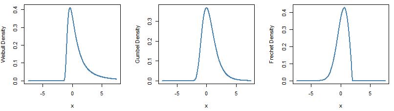
  , we get the Frechet distributions. When , we get the Weibull distributions.
At this stage its worth mentioning a couple of points. First, even though Fisher–Tippett–Gnedenko theorem tells us that the limiting distribution of belongs to one of three possible families of distributions we only need to consider GEV because it encompasses all three distributions. Secondly, the results stated up to this point relied on the assumption of existence of some normalizing constant and but we do not need to actually estimate them. We have the theoretical results justifying the use of the GEV distribution but when we try to fit the distribution to our data we are simply considering the three parameters (
, we get the Frechet distributions. When , we get the Weibull distributions.
At this stage its worth mentioning a couple of points. First, even though Fisher–Tippett–Gnedenko theorem tells us that the limiting distribution of belongs to one of three possible families of distributions we only need to consider GEV because it encompasses all three distributions. Secondly, the results stated up to this point relied on the assumption of existence of some normalizing constant and but we do not need to actually estimate them. We have the theoretical results justifying the use of the GEV distribution but when we try to fit the distribution to our data we are simply considering the three parameters ( )
)
Lets now have a look at what the three distributions look like. In R package fExtremes has function dgev to plot the GEV density.
require(fExtremes)
par(mfrow=c(1,3))
x <- seq(from = -7.5, to = 7.5, length.out = 550)

# plot Weibull
plot(x, dgev(x, xi = 0.5, mu = 0, beta =1),
     type = 'l', lty = 1, lwd = 2,
     col = 'steelblue', ylab = 'Density')

# plot Gumbel
plot(x, dgev(x, xi = 0, mu = 0, beta =1),
     type = 'l', lty = 1, lwd = 2,
     col = 'steelblue', ylab = 'Density')

# plot Frechet
plot(x, dgev(x, xi = -0.5, mu = 0, beta =1),
     type = 'l', lty = 1, lwd = 2,
     col = 'steelblue', ylab = 'Density')
Below are the density plots:
At this point I hope the main idea of Block Maxima approach to EVT are well understood and I will move on to playing with data and seeing how we can put the theory to work.
Data Fitting – Block Maxima:
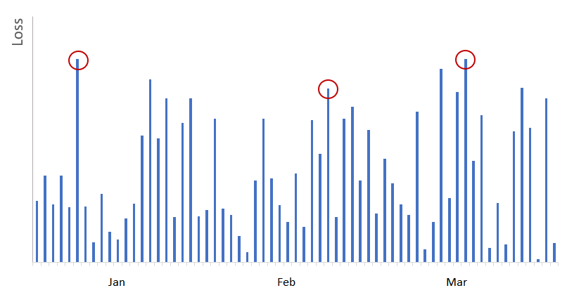
We now know that we want to fit a GEV distribution to some data set. The issue is how to do it. We are trying to model maxima so lets try the following. Lets take some historical data, break it into k blocks, and look at the maximum value in each block and consider that to be our sampled value that we are trying to model. Lets assume we are working with a financial time series and we are looking at daily returns. Furthermore assume we are trying to model loss distribution so we will look at only negative returns on a daily basis. Below is a stylized chart assuming looking at only losses (represented as positive values). We are looking at 3 months worth of data. We can break the data set into monthly blocks and take measure the maximum in each month. We highlight the three observations below in red. The three observations would be used to fit the GEV distribution.
Note: In below chart we only used three months to highlight the idea of what block maxima means. In reality we need a lot more data to infer our GEV parameters ().
In our example we will be working with daily returns on SPY. We can load n years worth of data and break it into monthly blocks. So we will have k=n/12 blocks. For this example we will use R’s quantmod package to load data for 13 years. We then calculate maximum daily loss for each month and also keep the day of the observation even though it is not necessary.
require(quantmod)
require(xts)

SPY_prices <- Ad(getSymbols('SPY',
                            from = '2006-01-01',
                            to = '2019-01-01',
                            auto.assign = FALSE))

returns_xts <- diff(log(SPY_prices), k = 1)[-1]*100  # Daily log returns

# below reverses sign of returns_xts so loss is a positive number
# then collect max value for each month

monthly_max_daily_loss <- do.call(rbind,
                                  lapply(split(x = -1*returns_xts, 'months'),
                                        function(x) x[which.max(x)]))
. We have the distribution function  which is the cumulative distribution. The density function is the derivative of this function
  .
.
 The log likelihood function is simply the product of the log of individual densities. When
  , we have:
 One of the conditions is that
 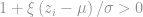 for all observations.
When , the log likelihood function is:
for all observations.
When , the log likelihood function is:

Since we are trying to maximize the likelihood, but our optimization routines are for minimization routines, we will implement the negative log likelihood function and minimize it. Mathematically the two are equivalent.
# likelihood function
gev_loglik <- function(params, data){
    mu <- params[1]; sigma <- params[2]; xi <- params[3]
    data <- coredata(data)
    m <- nrow(data)

    if((sigma <=0) | (xi <= -1)) return(1e6)  # if outside bounds return large value
    term1 <- -m*log(sigma)
    term2 <- (data-mu)/sigma

    # case xi = 0 (ie Gumbel distribution)
    if(abs(xi)<= .0001){
        result <- term1 - sum(term2) - sum(exp(-term2))
    } else {
        if(any(1+xi*term2 <= 0)) return(1e6)
        result <- term1 - (1+(1/xi))*sum(log(1+xi*term2))-sum((1+xi*term2)^(-1/xi))
    }
    return(-result)
}
Now let’s try to minimize the function:
my_gev_fit <- optim(par = c(1,1,.05), fn = gev_loglik, method = "Nelder-Mead", data = monthly_max_daily_loss)
my_gev_fit
$par
1.26096477678288   0.799888376043898   0.275120760011372
$value
235.677220980881
$counts
function   70
gradient   <NA>
$convergence
0
$message
NULL
We can compare this result with fExtremes’ gevFit function.
gevFit(coredata(monthly_max_daily_loss), block = 1, type = 'mle')
Title:
  GEV Parameter Estimation
Call:
  gevFit(x = coredata(monthly_max_daily_loss), block = 1, type = "mle")
Estimation Type:
   gev mle
Estimated Parameters:
        xi        mu      beta
 0.2751779 1.2611064 0.7999340
You can see that our estimated parameters are close.
Now that we have our estimated parameters, we can calculate various risk measures. For example, we can compute Value at Risk (VaR) and Expected Shortfall (ES).
In fact, VaR is easy to calculate. It is simply the output of the inverse cumulative distribution function (quantile function) at some alpha, , where
  .
.
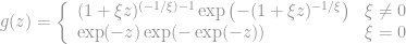
The inverse of the cumulative distribution function is given as:
![\hat{z}_{p}=\left\{\begin{array}{ll}{\mu-\frac{\dot{\sigma}}{\hat{\xi}}\left[1-y_{p}^{-\xi}\right],} & {\text { for } \hat{\xi} \neq 0} \\ {\hat{\mu}-\hat{\sigma} \log (- y_{p}),} & {\text { for } \hat{\xi}=0}\end{array}\right.](https://s0.wp.com/latex.php?latex=%5Chat%7Bz%7D_%7Bp%7D%3D%5Cleft%5C%7B%5Cbegin%7Barray%7D%7Bll%7D%7B%5Cmu-%5Cfrac%7B%5Cdot%7B%5Csigma%7D%7D%7B%5Chat%7B%5Cxi%7D%7D%5Cleft%5B1-y_%7Bp%7D%5E%7B-%5Cxi%7D%5Cright%5D%2C%7D+%26+%7B%5Ctext+%7B+for+%7D+%5Chat%7B%5Cxi%7D+%5Cneq+0%7D+%5C%5C+%7B%5Chat%7B%5Cmu%7D-%5Chat%7B%5Csigma%7D+%5Clog+%28-+y_%7Bp%7D%29%2C%7D+%26+%7B%5Ctext+%7B+for+%7D+%5Chat%7B%5Cxi%7D%3D0%7D%5Cend%7Barray%7D%5Cright.&bg=ffffff&fg=888888&s=0&c=20201002) where
where  .
.
The implementation is below:
GEV_VAR <- function(params, alpha = .05){
    # to vectorize the function we need vectors of estimated coefficients
    mu    <- rep(params[1], length(alpha))
    sigma <- rep(params[2], length(alpha))
    xi    <- rep(params[3], length(alpha))

    y <- -log(1-alpha)
    result <- ifelse(abs(xi) < 0.0001, mu -sigma*log(-y), mu -sigma/xi*(1-y^-xi))
    return(result)
}
Now we can extract our fitted coefficients and feed them into our VaR function and estimate the VaR at various alphas. Please note that in this implementation, alpha of 5% means it is the 95th percentile of the distribution.
my_fit_vals <- my_gev_fit$par
GEV_VAR(my_fit_vals, alpha = c(.05, .025, .01))
4.93706812468633 6.34878189965057 8.66305966965268
Let’s check our results versus fExtremes’ native quantile function using the fitted values from the gevFit function:
# lets check the results verus fExtremes' quantile function
qgev(p = 1- c(.05, .025, .01), xi = 0.2751779, mu = 1.2611064, beta = 0.7999340)
4.93682630963963 6.3484731241556 8.66265699310054
Our results are very close.
Finally, let’s write a function to get the Expected Shortfall (ES). And let’s calculate the ES at 1% level. We will implement a numerical integration here.
GEV_ES <- function(params, alpha = .05){
    my_fun <- function(x){GEV_VAR(x, params = params)}
    result <- 1/alpha * integrate(my_fun, lower = .00001, upper = alpha, stop.on.error = FALSE)$value
    return(result)
}

GEV_ES(my_fit_vals, alpha = .01)
12.49453391079
Notice that at 1% the VaR is 8.66% but the expected shortfall (conditional VaR) is much more significant, 12.50%.
Peak-Over-Threshold
Main idea:
A more common approach to EVT in finance is the so-called Peak-Over-Threshold (POT) method. It must be obvious to the reader that we have been very wasteful with our data up to this point. We discarded all observations in every month except for one extreme.
In the POT method, we instead retain all observations that exceed some value . For the moment, let’s avoid the discussion of how is selected, and just concentrate on the main idea.
Occasionally, we may observe multiple “extreme” observations in a given time block, and other months may be quiet. This may create instances where we under-represent the tail of the distribution when estimating the GEV model. For example, using Block Maxima method, we would’ve picked the losses circled in red (i.e. largest loss in each calendar month) to model tail distributions:
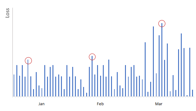
As shown in above graph, we would’ve ignored many extreme losses occurred in March, while using insignificant losses from January and February when we use Block Maxima method.
In POT we instead retain observations that exceed some threshold as shown below.
 are i.d.d. but now we want to know the distribution of given that it exceeds some value .
 The numerator is the probability that is greater than
  , and the denominator is the probability that is greater than .
Data Fitting – POT:
A theorem in EVT called Pickands-Balkema-de Haan states that if Block Maxima have approximately GEV distribution, the values in excess of some threshold (for a large enough threshold) has a limiting distribution given as below:
This distribution is referred as the Generalized Pareto Distribution (GPD).
Here, is the sahpe parameters, and  is defined as
  .
Please note that the parameter here is the same as the one in GEV distribution. And is a function of the sigma and mu parameters of GEV. In practice if we were to estimate either GEV or GPD distributions, the identities here would not be recovered because of numerical issues but the twos are inexorably linked.
.
Please note that the parameter here is the same as the one in GEV distribution. And is a function of the sigma and mu parameters of GEV. In practice if we were to estimate either GEV or GPD distributions, the identities here would not be recovered because of numerical issues but the twos are inexorably linked.
Like what we did for GEV, let’s plot the density functions using fExtremes package.
par(mfrow=c(1,3))
x <- seq(from = -7.5, to = 7.5, length.out = 550)


plot(x, dgpd(x, xi = 0.5, mu = 0, beta =1),
     type = 'l', lty = 1, lwd = 2,
     col = 'steelblue', ylab = 'Density')

plot(x, dgpd(x, xi = 0, mu = 0, beta =1),
     type = 'l', lty = 1, lwd = 2,
     col = 'steelblue', ylab = 'Density')

plot(x, dgpd(x, xi = -0.5, mu = 0, beta =1),
     type = 'l', lty = 1, lwd = 2,
     col = 'steelblue', ylab = 'Density')

 as
as  . Then the log likelihood function is given as:
 And in the special case when is equal to zero, the log likelihood function is given as:

gdp_loglik <- function(params, threshold, data){
    xi <- params[1]; tau <- params[2]
    data <- data - threshold # y = x-u
    data <- coredata(data[data >0]) # only need data that exceeds threshold
    m <- nrow(data)

    if((tau <=0) | (xi <= -1)) return(1e6)  # if outside bounds return large value
    term1 <- -m*log(tau)

    #  case xi = 0
    if(abs(xi) < 0.0001){
        result <- term1 - 1/tau *sum(data)
    } else {
        if(any(1+xi*data/tau <=0)) return(1e6)
        result <- term1 - (1+1/xi)*sum(log(1+xi*data/tau))
    }
    return(-result)
}
Now, let’s load some SPY data again and fit the parameters.
require(quantmod)
require(xts)

SPY_prices <- Ad(getSymbols('SPY',
                            from = '2006-01-01',
                            to = '2019-01-01',
                            auto.assign = FALSE))

returns_xts <- -1*diff(log(SPY_prices), k = 1)[-1]*100  # Daily log returns
names(returns_xts)<- 'SPY_Returns'
Using a threshold of 0.85 we can run our optimization.
my_threshold <- .85
#my_gpd_fit
my_gpd_fit <- optim(par = c(.5,.5),
                    fn = gdp_loglik,
                    method = "Nelder-Mead",
                    threshold = my_threshold,
                    data = returns_xts)
my_gpd_fit
$par
0.150591120379977   0.861181165068411
$value
476.579589960172
$counts
function 55
gradient <NA>
$convergence
0
$message
NULL
And let’s compare it to fExtremes package output.
gpdFit(coredata(returns_xts), u = my_threshold, type = 'mle')
Title:
   GPD Parameter Estimation
Call:
  gpdFit(x = coredata(returns_xts), u = my_threshold, type = "mle")
Estimation Method:
   gpd mle
Estimated Parameters:
        xi      beta
 0.1507411 0.8610883
Again, we are close.
Now that we have our estimated parameters, we can move on to calculating our two risk measures: VaR and ES.
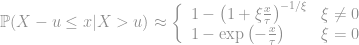
The quantile function is given as:
![\hat{z}_{p}=\left\{\begin{array}{ll}{u+\frac{\hat{\tau}}{\hat{\xi}}\left[\left( \frac{p}{\zeta_{u}} \right)^{-\xi}-1\right],} & {\text { for } \hat{\xi} \neq 0} \\ {u-\hat{\tau} \log \frac{p}{\zeta_{u}}} & {\text { for } \hat{\xi}=0}\end{array}\right.](https://s0.wp.com/latex.php?latex=%5Chat%7Bz%7D_%7Bp%7D%3D%5Cleft%5C%7B%5Cbegin%7Barray%7D%7Bll%7D%7Bu%2B%5Cfrac%7B%5Chat%7B%5Ctau%7D%7D%7B%5Chat%7B%5Cxi%7D%7D%5Cleft%5B%5Cleft%28+%5Cfrac%7Bp%7D%7B%5Czeta_%7Bu%7D%7D+%5Cright%29%5E%7B-%5Cxi%7D-1%5Cright%5D%2C%7D+%26+%7B%5Ctext+%7B+for+%7D+%5Chat%7B%5Cxi%7D+%5Cneq+0%7D+%5C%5C+%7Bu-%5Chat%7B%5Ctau%7D+%5Clog+%5Cfrac%7Bp%7D%7B%5Czeta_%7Bu%7D%7D%7D+%26+%7B%5Ctext+%7B+for+%7D+%5Chat%7B%5Cxi%7D%3D0%7D%5Cend%7Barray%7D%5Cright.&bg=ffffff&fg=888888&s=0&c=20201002) where
where  , which is the unconditional probability of observing variable above our chosen threshold. We simply take that as the number of observations exceeding our threshold as a ratio to total number of observations in our dataset.
GPD_VAR <- function(params, data, threshold, alpha = .05){
    n <- nrow(data)
    k <- sum(data > threshold)  # number of obs that exceed threshold
    # to vectorize the function we need vectors of estimated coefficients
    xi  <- rep(params[1], length(alpha))
    tau <- rep(params[2], length(alpha))

    result <- ifelse(abs(xi) < 0.0001, threshold - tau*log(alpha*n/k) ,
                                       threshold + tau/xi*((alpha*n/k)^-xi -1))
    return(result)

}
For GPD, there is a closed form for Expected Shortfall:

GPD_ES <- function(params, data, threshold, alpha = .05){
    # to vectorize the function we need vectors of estimated coefficients
    xi  <- rep(params[1], length(alpha))
    tau <- rep(params[2], length(alpha))
    VAR <- GPD_VAR(params, data, threshold, alpha)

    result <- VAR/(1-xi)+ (tau-xi*threshold)/(1-xi)
    return(result)
}
The outputs are
GPD_VAR(c(0.15059, 0.86118), coredata(returns_xts), my_threshold, .01)
GPD_ES(c(0.15059, 0.86118), coredata(returns_xts), my_threshold, .01)
3.69068499489364
5.20816036412762
And we can check this with the output of fExtremes package function gpdRiskMeasures.
gpdRiskMeasures(fextreme_gpd_fit, prob= c(.99))
        p quantile shortfall
beta 0.99 3.690996 5.209194
As you can see, our results are close to the output from fExtremes package.
Finally, a quick note on how to select the threshold u. This is more of an art than science. A common approach relies on Mean Excess Plots. The idea here is that for GPD, the mean excess value is a linear function of the threshold.
 With this knowledge, we can plot the average value that exceeds threshold for different values of . When the plot begins to look like a straight line, we take that as our value . To calculate
  for different values
  , we simply sum all values
  and divide by the number of observations where is greater than .
In fExtremes, there is a function mxfPlot that can do this for us.
mxfPlot(coredata(returns_xts), u = 0, cex = .5)
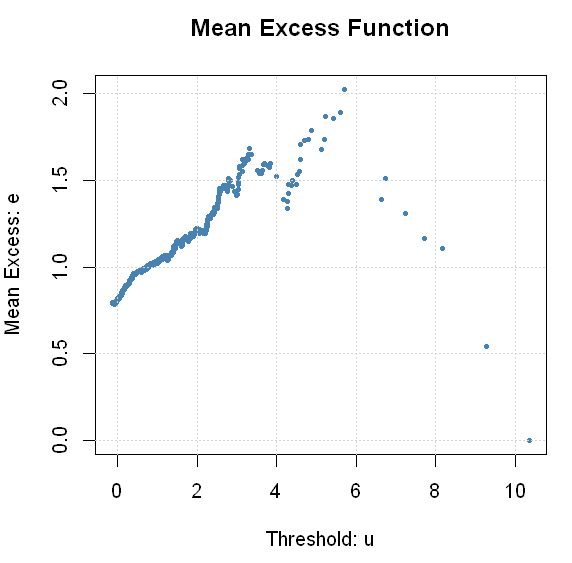
If you squint long enough, you might agree with me that a case can be made that mean excess is linear somewhere between 0.25-1.00. It seems like our initial choice of 0.85 wasn’t too bad. There are more methods that can assist us with the appropriate choice of threshold. You can consult some of the sources that are cited at the end of this post.
We covered a lot of the core concepts and introduced the main ideas behind EVT implementation. Hope you enjoyed.
Resources
- Good book with a dedicated chapter on EVT. I relied heavily on Chapter 6 for the discussion of MLE implementation in R. The author has an amazing blog that I discovered while finishing up this post. It is definitely worth checking out: https://freakonometrics.hypotheses.org/
- “An Introduction to Statistical Modeling of Extreme Values”
- Excellent article on EVT application in Finance.
- “Financial Risk Modelling and Portfolio Optimization in R” covers EVT in chapter 7. There is a lot of excellent material in this book in general, and is well worth the price.
- And just for fun, an interesting method to price catastrophe bonds based on EVT.

One thought on “Extreme Value Theory”