In previous post we showed a method of how to test for statistically significant seasonality in Excel. We also mentioned that the dummy regression approach can be applied to test other hypothesis. In this post we will use a similar approach to test for statistically different returns in selected securities conditional on the global business cycle.

To model the state of the global business cycle we use OECD`s Leading Indicator that is cyclically adjusted. We define one of four states based on whether the series is above or below 100 and if it increased or decreased in the month. The definitions are stated below in a tabular format:

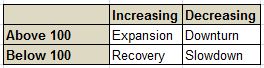
We again set up a column for each state. For example in column G the row is set to 1 if the OECD LI was above 100 and increased that month and 0 otherwise.

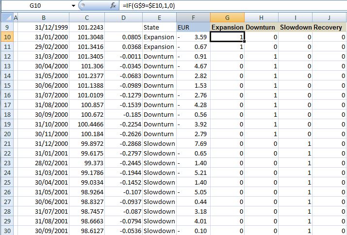
We can then run a regression procedure with Y equal to the monthly returns and Xs being the business cycle states.

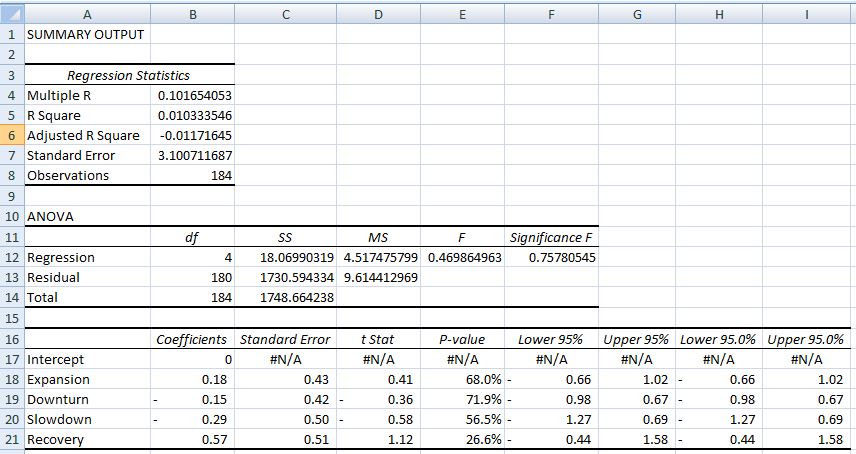
The output for EUR against USD looks like below. Note the high values of the p-value which indicates there is no statistically significant difference in monthly returns based on global business cycle state.

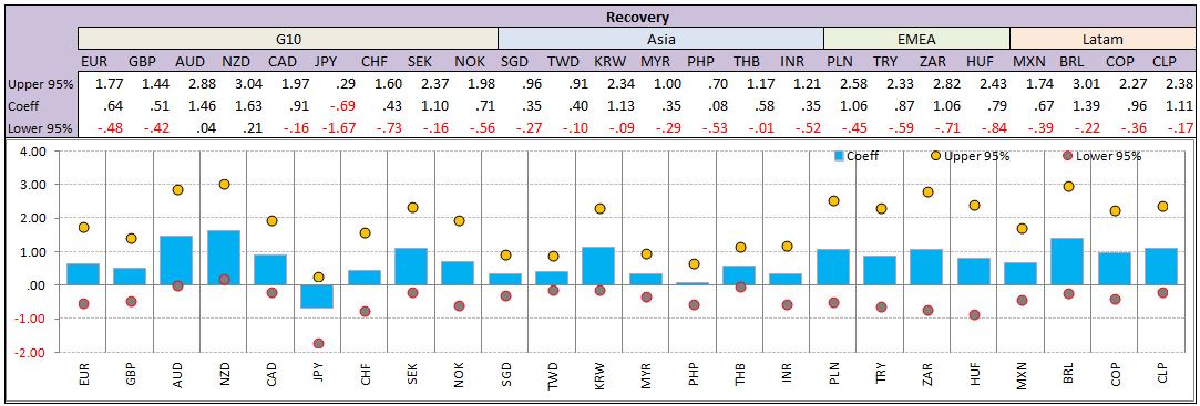
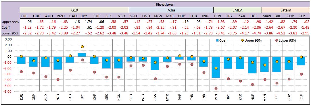
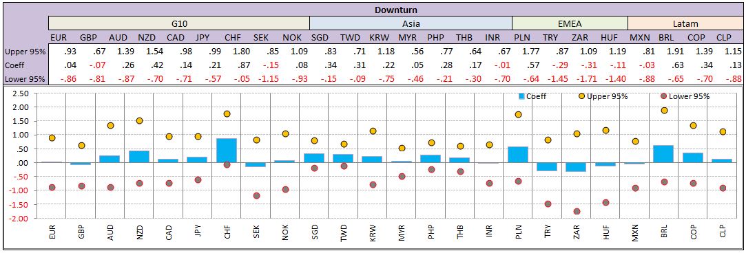
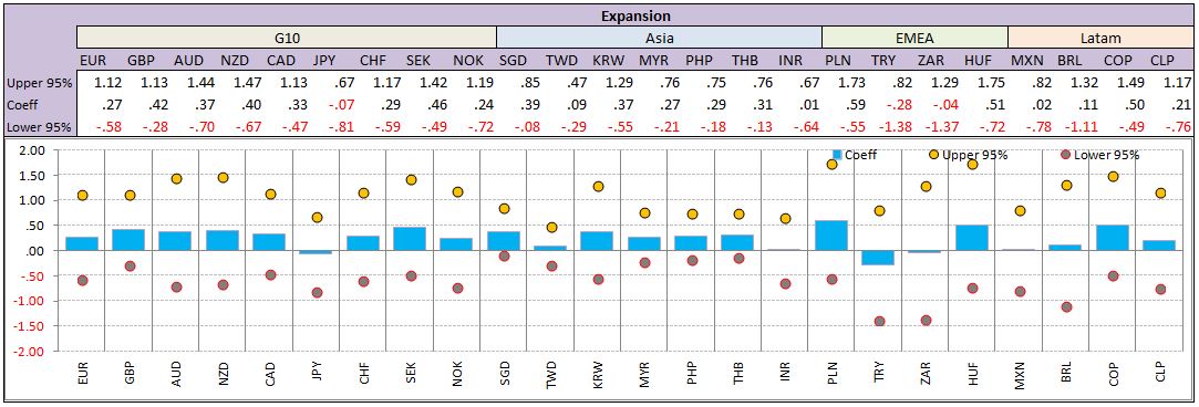
We can repeat this exercise for a selected list of securities. Below we check FX spot returns (excluding carry) for a list of currencies measured against USD for the last 12 years. We plot the coefficients and +/- 95% confidence levels to spot statistically significant returns. The results reveal strongest results for Recovery and Slowdown states.

In the case of Recovery state we can see that AUD, NZD, CAD, SEK, TWD, KRW, THB, and BRL have strong returns while JPY typically depreciates.

Below are results for the other three business cycle states

In addition to above analysis it would be helpful to look at transition probabilities from one business cycle state to another to make probabilistic assessment of expected returns.