In this post we will discuss a popular class of neural networks, Artificial Feedforward Neural Network (ANN) which consists of input data, one or more hidden layers consisting of processing units and an output layer which returns the value of an estimated target value. An example of a processing unit is shown below.

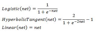
The processing unit which is also referred to as a node or a neuron (blue) has a number of inputs (orange) that have a weight associated with it. The weighted value of the inputs produces a net charge for the processing unit. The net value is then processed via some activation function to produce a neuron output. If a bias input is included then its value is 1. To show a computational example let’s assume bias = 1, x2 = -1, x3 = -1, while the weight from bias node to the processing neuron is .1, the weight from the second input node to the processing neuron is .2 and the weight of the third input node connection to the processing neuron is .3. Now we can compute the net charge of the processing neuron (1)x(.1)+(-1)x(.2)+(-1)x(.3) which is -.40. Finally to compute the output value of the processing neuron we need to pass .4 into some activation function. The three most popular activation functions used are the Logistic, Hyperbolic Tangent, and Linear function. Each is given below:

And this is all there is to it to computing the value of a node.

An ANN typically has an input layer where the node values are simply place holders for the data that you want your network to use as information to learn to predict or classify some output. For instance if you are building a network that is predicting a particular stock’s price then the input layer will consist of data that you think will allow you to predict a stock. Some candidate variables would be the broad market valuation, the company’s recent returns, stocks volatility, valuation of competitor firms, etc. Each of the input nodes is connected to each node of the hidden layer. ANNs can have multiple hidden layers. These layers compute neuron values just as shown above. The output (or node values) of the hidden layer is fed forward into the following layer. The network ends with a final output layer. The output layer can have multiple neurons. The output neuron value is what we are trying to attain after the modelling exercise is complete. In the example of a stock forecasting neural network, there would be a single output neuron which produces the stock price forecast.

The goal of setting up a neural network and to train it is to end up with a network that takes in some data as an input and produce an estimated output that matches closely some desired value (this is called supervised training and we won’t be covering unsupervised training since it is rarely used in finance). The process of training a network is basically an exercise of adjusting all the connecting weights in the ANN to achieve predictions or estimates of some variable(s).

Below is an example of a fully connected (connections from each input node to the nodes of the following layer) with a single hidden layer and one output neuron.

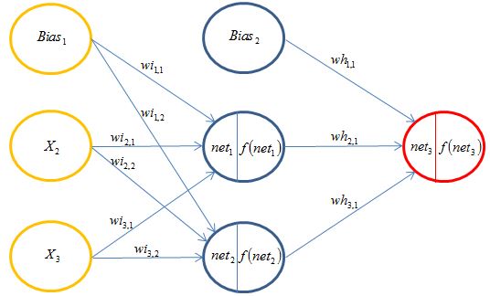We can add more neurons to any layer and can add more hidden layers. Below is an example of a network with 1 input layer with 2 nodes, 2 hidden layers with 3 nodes in the first layer and 2 nodes in the second hidden layer, and an output layer with 2 output nodes and a bias input into each node of the network. It is modeller’s decision on how many nodes and hidden layer to use. Multiple variants are usually tried and checked against a validation set (data that is not used to train the weights but only to check how the model fits data).

There are many ways to train a network. Most popular method seems to be the back propagation method. This method is sometimes referred to as the general delta method or the gradient method. The idea is to set up an error measure or a cost function and then to systematically adjust the weights until the error function is minimized. First we will derive the back propagation algorithm and then take you through one loop of the computations. As we go along we will also explain the main snippets of the code that perform the calculations.

Back Propagation Derivation

Typically an error function is set up for the error node as below:

So the error function is simply the sum of squared error for each of the output neurons. We multiply by a scalar .5 just to simply the derivation since we will be taking the derivative of the error function. It makes no real difference if we were to leave it out.

Now that we have our error function that we wish to minimize we need to have a systematic method that adjusts the weights to achieve that goal. First working with the output nodes we can use calculus to derive the derivative of the error function with respect to each weight that connects into the output neurons.

What we need is to calculate:

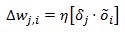
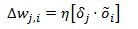
We can then adjust our weight by adding to the current weight an adjustment based on the computed gradient as:

where eta is called a learning parameter and is specified by the modeller and is often kept constant. Learning rate needs to be between 0 and 1. We have a negative sign in front of the formula because we are trying to minimize the error function.

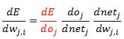
To calculate the necessary gradient we need to use the Chain Rule of calculus. We have:

For now let’s assume we are working with a single output node to make the notation lighter. Lets calculate the first derivative of the above equation. We have:

We can move on to the second derivative in the main equation

We can now compute the final derivative in the function

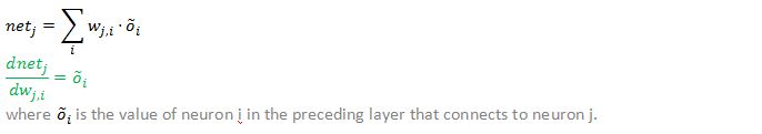
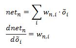
Recall that the net charge of the neuron is simply the weighted sum of the preceding network’s neuron values and the connection weights. So we have:

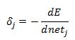
At this stage lets define a variable delta as:

So we have:

Now we can combine our results

substituting this into our weight adjustment formula we have:

Things get a little more complicated when we turn our attention to the hidden layer. The main difficulty is the notation which gets cumbersome so hopefully our numerical example later on will help with the exposition.

The main issue with deriving the adjustment for the weights in the lower layers in the network is that we do not know what the error for each node is. This is obvious if we spend a minute thinking about it. We have hidden neurons that propagate signals through the network until we reach the output node and only then can compare the estimated value (neuron output) to some target value and compute the error. We do not know how much the hidden neurons contributed to the error since we don’t know what the target output for each hidden neuron should be.

A clever way around this problem is to recognize that each node in the hidden layer contributes a value to the output node via the net value that feeds into the output node activation function. In the below diagram we highlight this. The last node in the second hidden layer has an output value which then feeds forward into the calculation of net charge of each output neuron.

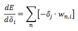
With that in mind lets differentiate the error function with respect to the output of a hidden node. Via Chain Rule we have:

where n is the number of output nodes.

This formula simply states that the derivative of the error function with respect to hidden layer neuron i output is a function of the partial derivative of the error function with respect to the net charge of that output neuron times the derivative of the net charge of the output neuron with respect to its input (which is the output of the node we are analyzing).

Notice that we already computed one of the partial derivatives in the previous step. We had calculated:

So we have

And calculating the derivative of the net function with respect to its input value we get:

Therefore what we have so far for the hidden layer is:

Let’s remember that what we are looking for are values to input into our weights update formula

where

and via Chain Rule

we already have

and we know that

so updating our formula we have:

which we can plug into our weight update formula

Hopefully at this point you can understand why this is called a back propagation algorithm. We compute the error of the output nodes and then work our way backwards through the neural network and adjust the weights.

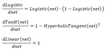
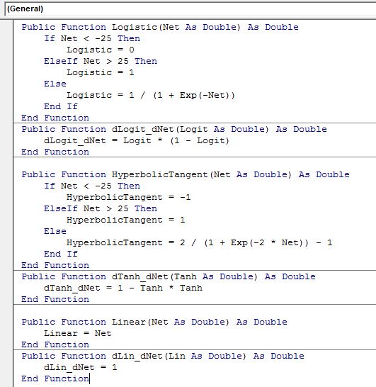
Now it’s time for us to discuss activation functions and their derivatives. As we mentioned earlier the most common three activation functions are Logistic, Hyperbolic Tangent, and Linear. It is typical for a given layer to use the same type of activation function. Also, hidden layers always uses non linear activation functions. Therefore, linear activation function can be used for the output layer but not hidden layers. First derivatives of each function with respect to its input are given below:

We should also mention here that what was shown was a sequential update rule for the network weights. This means we present a pattern of data to the input layers and then propagate forward through the network. After we compute the output values we compare them to our target values and calculate the error. Once we know the error we use above equations to calculate the weight adjustments. Finally, once we have the weight adjustments we can adjust the weights and present another pattern to the network and repeat the process. These steps are repeated until a maximum number of iterations is reached or until our error function has reached some minimum.

An alternative method to train a network, and the one we implemented below, is called a batch training method. We present each training pattern to the network and compute the weight adjustment for all instances of the training data. After we presented all the training data we sum across all the weight changes for a given weight and use this sum to update the weight. At this stage we have completed what is called a single epoch of the training cycle. We then repeat this process and again present all the training data to the network and for each training instance we calculate the weight adjustment value and again sum across all the weight. We then update the network weights and repeat as necessary. This process is repeated until the error function is minimized or until we reach a maximum number of epochs.

Numerical Example

Most common problem presented in introductory exposition of an ANN is the XOR function.

We need to decide on a network topology for this problem. We will use a single hidden layer with 2 nodes and a single output node. Each node in the network will have a bias threshold. Also, we will use logistic function as the activation function in the hidden layer and the hyperbolic function as the activation function for the output layer. As we work our way through the example we will present parts of VBA code to help with its interpretation.

Firs we need to assign weight for the network. We will use below:

The network looks like below with the first training instance presented to the input nodes:

At this stage we can calculate the value of the hidden node neurons. The bias node is always assigned a value of 1. The second neuron in the hidden layer has a net charge of (1)x(.1)+(-1)x(.2)+(-1)x(.3)=-.4. The neuron value using the logistic function is equal to .4013. Moving on to the second neuron in the hidden layer we get a net charge value of (1)x(-.3)+(-1)x(-.2)+(-1)x(-.1) = 0. The value after feeding the net charge into the logistic function yields .5000. What we have so far then is:

We can now proceed to calculate the network output. The output node’s net charge is (1)x(-.35)+(.4013)x(.35)+(.5000)x(.15)=-.1345. Passing this value through the hyperbolic tangent function returns -.1337. So at this point we have completed a single pass through the network and compute the error. Since XOR returns -1 which is out target value our error value is (-1)+(-.1337) = -.8663.

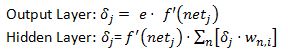
At this stage we need to calculate the deltas for each node starting from the output neuron. Lets remind ourselves that the delta formulas are:

Starting with the output node we have the error value of -.8663 and we know that the derivative of the hyperbolic tangent function is 1-(-.1337)²= .9821. The product of these two values is -.8508.

Moving on to the hidden layer’s first node we can calculate the derivative of the activation function with respect to its net as .4013x(1-.4013) = .2403. We can now multiply this value by the output node’s delta and the weight from the first hidden layer’s first node to the output layer, .2403x(-.8508)x.35= -.0715. Similarly for the second node in the hidden layer we have .5000x(1-.5000)x(-.8508)x.15 = -.0319.

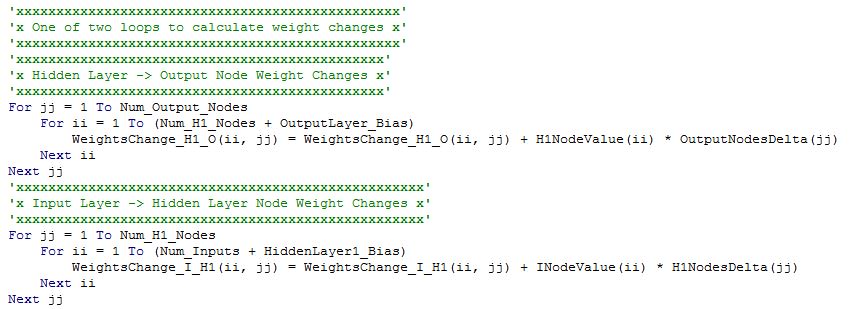
Now that we have all the deltas we can calculate our weight changes using formula

You have probably noticed that we left out the learning rate parameter. That is the case because we will update our weights only after we complete a full epoch using all the training data. It is this accumulated weight change that will be multiplied by the learning rate and then added to the current weights (batch vs sequential training).

We now have:

At this point we have completed one epoch. We now need to pass the other three training samples and repeat exactly the same calculations. After we have done that we will have a cumulated sum for each weight change. We then add the weight change multiplied by the learning rate to the weights and repeat the calculations.

In the code above we use a momentum rate. This is a slight change to what we discussed in the main part of the post. At times a momentum is used to calculate the new weights. The update formula is equal to:

This is a modification and adds alpha (momentum rate) multiplied by previous weight change calculation.

If we set alpha to zero in the code then our update rule is identical to what we discussed in the derivation of backpropagaton part of the post.

After we train the network we can see how the average square error evolves with each epoch. Below is the profile.

We can see that the neural network has learned and fits the data well:

Full VBA Code

To use the code in a workbook you will need to four tabs with the following names:

-Control

-DataInput

-TrainingResults

-Trained_NetworkWeights

On the control tab we need the following inputs along with a macro button that will call our main macro:

By reading the code we can easily understand what ranges in this sheet have range names assigned.

On the DataInput sheet the target output needs to be in a column that is to the left to the input values. Input values need to be grouped together with no empty columns between them.

The code that is presented below works only with a single hidden layer. It should not be too difficult to write another macro with additional hidden layers. We simply need to add layers to the feedforward code, delta calculations, and weights update part of the procedure.

We first need user defined functions for the activation functions and their derivatives:

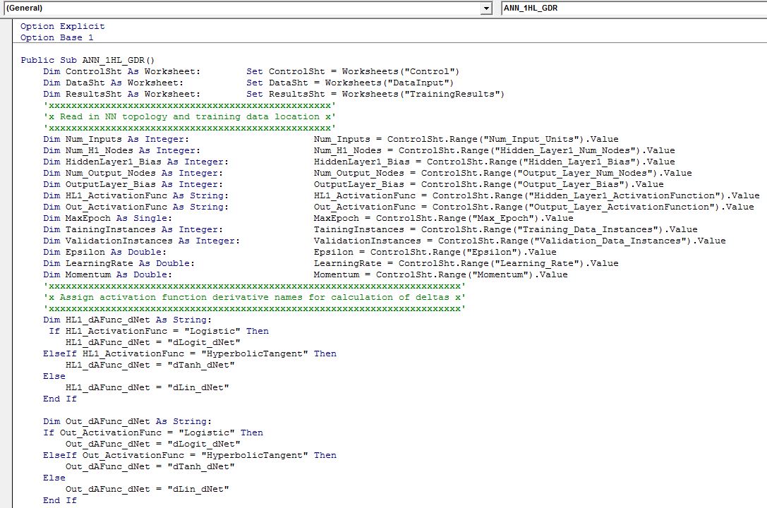
The main procedure for a fully connected ANN with a single hidden layer is below:

That’s all that we will say about neural networks here. Hopefully you find this post helpful.

Some Useful Resources:

1) Robert Schalkoff excellent book http://www.amazon.com/Artificial-Neural-Networks-Robert-Schalkoff/dp/007057118X

2) Nong Ye has a good discussion of neural networks but the worked example has errors so beware http://www.amazon.com/Data-Mining-Theories-Algorithms-Ergonomics/dp/1439808384/ref=sr_1_4?s=books&ie=UTF8&qid=1439459225&sr=1-4&keywords=nong+ye

3) Simon Hayakin’s book is excellent on ANN http://www.amazon.com/Data-Mining-Theories-Algorithms-Ergonomics/dp/1439808384/ref=sr_1_4?s=books&ie=UTF8&qid=1439459225&sr=1-4&keywords=nong+ye

4) Jeff Heaton’s two books on ANN math and implementation were helpful http://www.heatonresearch.com/

5) Christian Dunis discusses ANN model for FX forecasting. He also has papers published on the subject. http://as.wiley.com/WileyCDA/WileyTitle/productCd-0470848855.html a list of his research publications is available at http://www.dunis.co.uk/publications.html

 

VBA:

Option Explicit
Option Base 1

Public Sub ANN_1HL_GDR()
Dim ControlSht As Worksheet:        Set ControlSht = Worksheets(“Control”)
Dim DataSht As Worksheet:           Set DataSht = Worksheets(“DataInput”)
Dim ResultsSht As Worksheet:        Set ResultsSht = Worksheets(“TrainingResults”)
‘xxxxxxxxxxxxxxxxxxxxxxxxxxxxxxxxxxxxxxxxxxxxxxxxxx’
‘x Read in NN topology and training data location x’
‘xxxxxxxxxxxxxxxxxxxxxxxxxxxxxxxxxxxxxxxxxxxxxxxxxx’
Dim Num_Inputs As Integer:                      Num_Inputs = ControlSht.Range(“Num_Input_Units”).Value
Dim Num_H1_Nodes As Integer:                    Num_H1_Nodes = ControlSht.Range(“Hidden_Layer1_Num_Nodes”).Value
Dim HiddenLayer1_Bias As Integer:               HiddenLayer1_Bias = ControlSht.Range(“Hidden_Layer1_Bias”).Value
Dim Num_Output_Nodes As Integer:                Num_Output_Nodes = ControlSht.Range(“Output_Layer_Num_Nodes”).Value
Dim OutputLayer_Bias As Integer:                OutputLayer_Bias = ControlSht.Range(“Output_Layer_Bias”).Value
Dim HL1_ActivationFunc As String:               HL1_ActivationFunc = ControlSht.Range(“Hidden_Layer1_ActivationFunction”).Value
Dim Out_ActivationFunc As String:               Out_ActivationFunc = ControlSht.Range(“Output_Layer_ActivationFunction”).Value
Dim MaxEpoch As Single:                         MaxEpoch = ControlSht.Range(“Max_Epoch”).Value
Dim TainingInstances As Integer:                TainingInstances = ControlSht.Range(“Training_Data_Instances”).Value
Dim ValidationInstances As Integer:             ValidationInstances = ControlSht.Range(“Validation_Data_Instances”).Value
Dim Epsilon As Double:                          Epsilon = ControlSht.Range(“Epsilon”).Value
Dim LearningRate As Double:                     LearningRate = ControlSht.Range(“Learning_Rate”).Value
Dim Momentum As Double:                         Momentum = ControlSht.Range(“Momentum”).Value
‘xxxxxxxxxxxxxxxxxxxxxxxxxxxxxxxxxxxxxxxxxxxxxxxxxxxxxxxxxxxxxxxxxxxxxxxxx’
‘x Assign activation function derivative names for calculation of deltas x’
‘xxxxxxxxxxxxxxxxxxxxxxxxxxxxxxxxxxxxxxxxxxxxxxxxxxxxxxxxxxxxxxxxxxxxxxxxx’
Dim HL1_dAFunc_dNet As String:
If HL1_ActivationFunc = “Logistic” Then
HL1_dAFunc_dNet = “dLogit_dNet”
ElseIf HL1_ActivationFunc = “HyperbolicTangent” Then
HL1_dAFunc_dNet = “dTanh_dNet”
Else
HL1_dAFunc_dNet = “dLin_dNet”
End If

Dim Out_dAFunc_dNet As String:
If Out_ActivationFunc = “Logistic” Then
Out_dAFunc_dNet = “dLogit_dNet”
ElseIf Out_ActivationFunc = “HyperbolicTangent” Then
Out_dAFunc_dNet = “dTanh_dNet”
Else
Out_dAFunc_dNet = “dLin_dNet”
End If
‘xxxxxxxxxxxxxxxxxxxxxxxxxxxxxxxxxxxxxxxxxx’
‘x Prepare output sheets for model output x’
‘xxxxxxxxxxxxxxxxxxxxxxxxxxxxxxxxxxxxxxxxxx’
ControlSht.Range(“Hidden_Layer1_Num_Nodes”).Offset(ControlSht.Range(“Num_Hidden_Layers”).Value, 0) _
.Resize(5 – ControlSht.Range(“Num_Hidden_Layers”).Value, 3).ClearContents ‘Removes superfluous hidden layer data

ResultsSht.Range(“B3”).Resize(ResultsSht.Range(“C:C”). _
Cells.SpecialCells(xlCellTypeConstants).Count, 3).ClearContents ‘ remove MSE data from TrainingResults tab

‘xxxxxxxxxxxxxxxxxxxxxxxxxxxxxxxxxxxxxxxxxxxxxxxxx’
‘x Count number of input nodes and create arrays x’
‘xxxxxxxxxxxxxxxxxxxxxxxxxxxxxxxxxxxxxxxxxxxxxxxxx’
Dim NumWghts_I_H1 As Integer:    NumWghts_I_H1 = (Num_Inputs + HiddenLayer1_Bias) * Num_H1_Nodes
ReDim Weights_I_H1(Num_Inputs + HiddenLayer1_Bias, Num_H1_Nodes) As Double ‘ weight from input i to node j
ReDim WeightsChange_I_H1(Num_Inputs + HiddenLayer1_Bias, Num_H1_Nodes) As Double ‘ gradient based weight adjustment
ReDim WeightsChange_I_H1_Prev(Num_Inputs + HiddenLayer1_Bias, Num_H1_Nodes) As Double ‘ used if momentum is required

‘xxxxxxxxxxxxxxxxxxxxxxxxxxxxxxxxxxxxxxxxxxxxxxxxxxxxxxxx’
‘x Count number of hidden layer nodes and create arrays x’
‘xxxxxxxxxxxxxxxxxxxxxxxxxxxxxxxxxxxxxxxxxxxxxxxxxxxxxxxx’
Dim NumWghts_H1_O As Integer:    NumWghts_H1_O = (Num_H1_Nodes + OutputLayer_Bias) * Num_Output_Nodes
ReDim Weights_H1_O(Num_H1_Nodes + OutputLayer_Bias, Num_Output_Nodes) As Double ‘ weight from node i to output node j
ReDim WeightsChange_H1_O(Num_H1_Nodes + OutputLayer_Bias, Num_Output_Nodes) As Double
ReDim WeightsChange_H1_O_Prev(Num_H1_Nodes + OutputLayer_Bias, Num_Output_Nodes) As Double

‘xxxxxxxxxxxxxxxxxxxxxx’
‘x Initialise weights x’
‘xxxxxxxxxxxxxxxxxxxxxx’
Dim ii As Integer:          ii = 1
Dim jj As Integer:          jj = 1
For jj = 1 To Num_H1_Nodes
For ii = 1 To (Num_Inputs + HiddenLayer1_Bias)
Weights_I_H1(ii, jj) = Rnd – 0.5
Next ii
Next jj
For jj = 1 To Num_Output_Nodes
For ii = 1 To (Num_H1_Nodes + OutputLayer_Bias)
Weights_H1_O(ii, jj) = Rnd – 0.5
Next ii
Next jj
‘xxxxxxxxxxxxxxxxxxxxxxxxxxxxxxxxxxxxxxxxxxxxxx’
‘x Starting weights to replicate blog example x’
‘xxxxxxxxxxxxxxxxxxxxxxxxxxxxxxxxxxxxxxxxxxxxxx’
‘    Weights_I_H1(1, 1) = 0.1:   Weights_I_H1(1, 2) = -0.3:  Weights_H1_O(1, 1) = -0.35
‘    Weights_I_H1(2, 1) = 0.2:   Weights_I_H1(2, 2) = -0.2:  Weights_H1_O(2, 1) = 0.35
‘    Weights_I_H1(3, 1) = 0.3:   Weights_I_H1(3, 2) = -0.1: Weights_H1_O(3, 1) = 0.15

‘xxxxxxxxxxxxxxxxxxxxxxxxxxxxxxxxxxxxxxxxxxxxxxxxx’
‘x Declaration of counters and summation holders x’
‘xxxxxxxxxxxxxxxxxxxxxxxxxxxxxxxxxxxxxxxxxxxxxxxxx’
Dim Epoch As Single:        Epoch = 1
Dim Obs As Integer:         Dim Obs_Val As Integer
Dim TempNet As Double:      Dim TempDeltaSum As Double
Dim AvgSqrError As Double:  Dim AvgSqrError_Val As Double

‘xxxxxxxxxxxxxxxxxxxxxxxxxxxxxxxxxxxxxxxxxxxxxxxxxxxxxxxxxxxxxxxxxxxxxxxxxxxxxxxxxxxxxxxxxxxxxxxxxxxxxxxxx’
‘x This is the main loop. Network is trained until maximum Epochs is reached or MSE converged to Epsilon x’
‘xxxxxxxxxxxxxxxxxxxxxxxxxxxxxxxxxxxxxxxxxxxxxxxxxxxxxxxxxxxxxxxxxxxxxxxxxxxxxxxxxxxxxxxxxxxxxxxxxxxxxxxxx’
For Epoch = 1 To MaxEpoch
‘xxxxxxxxxxxxxxxxxxxxxxxxxxxxxxxxxxxxxxxxxxxxxxxxxxxxxxxxxxxxxxxxxxxxxxxxxxxxxxxxxxxxx’
‘x  Model uses Batch Training Mode. For each sample we loop through:                 x’
‘x         1) Loads in Training Set                                                  x’
‘x         2) Feedforward the training set through network                           x’
‘x         3) Calculates error                                                       x’
‘x         4) Calculates deltas (dError/dNet)                                        x’
‘x         5) Calculates weight change                                               x’
‘xxxxxxxxxxxxxxxxxxxxxxxxxxxxxxxxxxxxxxxxxxxxxxxxxxxxxxxxxxxxxxxxxxxxxxxxxxxxxxxxxxxxx’
For Obs = 1 To TainingInstances
‘xxxxxxxxxxxxxxxxxxxxxxx’
‘x Loads Target Output x’
‘xxxxxxxxxxxxxxxxxxxxxxx’
ReDim TargetNodeValue(Num_Output_Nodes) As Double
For ii = 1 To Num_Output_Nodes
TargetNodeValue(ii) = DataSht.Range(ControlSht.Range(“Target_Data_Range”).Value).Offset(Obs – 1, ii – 1).Value
Next ii

‘xxxxxxxxxxxxxxxxxxxxxxxxxxxxxxxxxxxxxxxxxxxxxxxxxxxxxxxxxxxxx’
‘x Loads Input Nodes and incudes bias node value if selected x’
‘xxxxxxxxxxxxxxxxxxxxxxxxxxxxxxxxxxxxxxxxxxxxxxxxxxxxxxxxxxxxx’
ReDim INodeValue(Num_Inputs + HiddenLayer1_Bias) As Double
If HiddenLayer1_Bias = 1 Then
INodeValue(1) = 1#
End If
For ii = (1 + HiddenLayer1_Bias) To (Num_Inputs + HiddenLayer1_Bias)
INodeValue(ii) = DataSht.Range(ControlSht.Range(“Input_Data_Range”).Value).Offset(Obs – 1, ii – 1 – HiddenLayer1_Bias).Value
Next ii

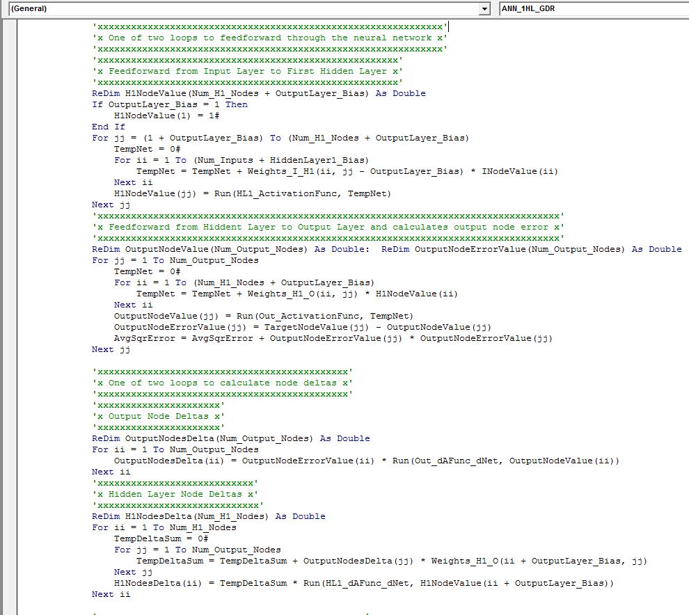
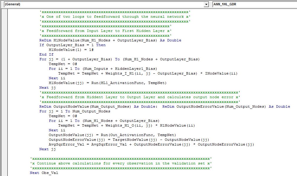
‘xxxxxxxxxxxxxxxxxxxxxxxxxxxxxxxxxxxxxxxxxxxxxxxxxxxxxxxxxxxxxx’
‘x One of two loops to feedforward through the neural network x’
‘xxxxxxxxxxxxxxxxxxxxxxxxxxxxxxxxxxxxxxxxxxxxxxxxxxxxxxxxxxxxxx’
‘xxxxxxxxxxxxxxxxxxxxxxxxxxxxxxxxxxxxxxxxxxxxxxxxxxxxxx’
‘x Feedforward from Input Layer to First Hidden Layer x’
‘xxxxxxxxxxxxxxxxxxxxxxxxxxxxxxxxxxxxxxxxxxxxxxxxxxxxxx’
ReDim H1NodeValue(Num_H1_Nodes + OutputLayer_Bias) As Double
If OutputLayer_Bias = 1 Then
H1NodeValue(1) = 1#
End If
For jj = (1 + OutputLayer_Bias) To (Num_H1_Nodes + OutputLayer_Bias)
TempNet = 0#
For ii = 1 To (Num_Inputs + HiddenLayer1_Bias)
TempNet = TempNet + Weights_I_H1(ii, jj – OutputLayer_Bias) * INodeValue(ii)
Next ii
H1NodeValue(jj) = Run(HL1_ActivationFunc, TempNet)
Next jj
‘xxxxxxxxxxxxxxxxxxxxxxxxxxxxxxxxxxxxxxxxxxxxxxxxxxxxxxxxxxxxxxxxxxxxxxxxxxxxxxxxxxx’
‘x Feedforward from Hiddent Layer to Output Layer and calculates output node error x’
‘xxxxxxxxxxxxxxxxxxxxxxxxxxxxxxxxxxxxxxxxxxxxxxxxxxxxxxxxxxxxxxxxxxxxxxxxxxxxxxxxxxx’
ReDim OutputNodeValue(Num_Output_Nodes) As Double:  ReDim OutputNodeErrorValue(Num_Output_Nodes) As Double
For jj = 1 To Num_Output_Nodes
TempNet = 0#
For ii = 1 To (Num_H1_Nodes + OutputLayer_Bias)
TempNet = TempNet + Weights_H1_O(ii, jj) * H1NodeValue(ii)
Next ii
OutputNodeValue(jj) = Run(Out_ActivationFunc, TempNet)
OutputNodeErrorValue(jj) = TargetNodeValue(jj) – OutputNodeValue(jj)
AvgSqrError = AvgSqrError + OutputNodeErrorValue(jj) * OutputNodeErrorValue(jj)
Next jj

‘xxxxxxxxxxxxxxxxxxxxxxxxxxxxxxxxxxxxxxxxxxxxx’
‘x One of two loops to calculate node deltas x’
‘xxxxxxxxxxxxxxxxxxxxxxxxxxxxxxxxxxxxxxxxxxxxx’
‘xxxxxxxxxxxxxxxxxxxxxx’
‘x Output Node Deltas x’
‘xxxxxxxxxxxxxxxxxxxxxx’
ReDim OutputNodesDelta(Num_Output_Nodes) As Double
For ii = 1 To Num_Output_Nodes
OutputNodesDelta(ii) = OutputNodeErrorValue(ii) * Run(Out_dAFunc_dNet, OutputNodeValue(ii))
Next ii
‘xxxxxxxxxxxxxxxxxxxxxxxxxxxx’
‘x Hidden Layer Node Deltas x’
‘xxxxxxxxxxxxxxxxxxxxxxxxxxxxx’
ReDim H1NodesDelta(Num_H1_Nodes) As Double
For ii = 1 To Num_H1_Nodes
TempDeltaSum = 0#
For jj = 1 To Num_Output_Nodes
TempDeltaSum = TempDeltaSum + OutputNodesDelta(jj) * Weights_H1_O(ii + OutputLayer_Bias, jj)
Next jj
H1NodesDelta(ii) = TempDeltaSum * Run(HL1_dAFunc_dNet, H1NodeValue(ii + OutputLayer_Bias))
Next ii

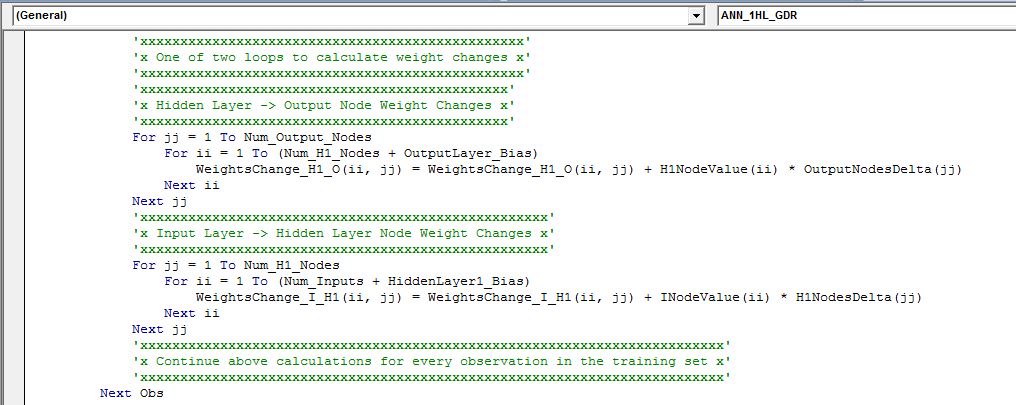
‘xxxxxxxxxxxxxxxxxxxxxxxxxxxxxxxxxxxxxxxxxxxxxxxx’
‘x One of two loops to calculate weight changes x’
‘xxxxxxxxxxxxxxxxxxxxxxxxxxxxxxxxxxxxxxxxxxxxxxxx’
‘xxxxxxxxxxxxxxxxxxxxxxxxxxxxxxxxxxxxxxxxxxxxxx’
‘x Hidden Layer -> Output Node Weight Changes x’
‘xxxxxxxxxxxxxxxxxxxxxxxxxxxxxxxxxxxxxxxxxxxxxx’
For jj = 1 To Num_Output_Nodes
For ii = 1 To (Num_H1_Nodes + OutputLayer_Bias)
WeightsChange_H1_O(ii, jj) = WeightsChange_H1_O(ii, jj) + H1NodeValue(ii) * OutputNodesDelta(jj)
Next ii
Next jj
‘xxxxxxxxxxxxxxxxxxxxxxxxxxxxxxxxxxxxxxxxxxxxxxxxxxx’
‘x Input Layer -> Hidden Layer Node Weight Changes x’
‘xxxxxxxxxxxxxxxxxxxxxxxxxxxxxxxxxxxxxxxxxxxxxxxxxxx’
For jj = 1 To Num_H1_Nodes
For ii = 1 To (Num_Inputs + HiddenLayer1_Bias)
WeightsChange_I_H1(ii, jj) = WeightsChange_I_H1(ii, jj) + INodeValue(ii) * H1NodesDelta(jj)
Next ii
Next jj
‘xxxxxxxxxxxxxxxxxxxxxxxxxxxxxxxxxxxxxxxxxxxxxxxxxxxxxxxxxxxxxxxxxxxxxxxxx’
‘x Continue above calculations for every observation in the training set x’
‘xxxxxxxxxxxxxxxxxxxxxxxxxxxxxxxxxxxxxxxxxxxxxxxxxxxxxxxxxxxxxxxxxxxxxxxxx’
Next Obs

‘xxxxxxxxxxxxxxxxxxxxxxxxxxxxxxxxxxxxxxxxxxxxxxxxxxxxxxxxxxxxxxxxxxxxxxxxxxxxxxxxxxxxxxxxxxxxxxxxxxxxxxxxxxxxxxxxx’
‘x This is the main loop that will calculate MSE for validation set to check the out of sample fit of the model  x’
‘xxxxxxxxxxxxxxxxxxxxxxxxxxxxxxxxxxxxxxxxxxxxxxxxxxxxxxxxxxxxxxxxxxxxxxxxxxxxxxxxxxxxxxxxxxxxxxxxxxxxxxxxxxxxxxxxx’
For Obs_Val = 1 To ValidationInstances
‘xxxxxxxxxxxxxxxxxxxxxxx’
‘x Loads Target Output x’
‘xxxxxxxxxxxxxxxxxxxxxxx’
ReDim TargetNodeValue(Num_Output_Nodes) As Double
For ii = 1 To Num_Output_Nodes
TargetNodeValue(ii) = DataSht.Range(ControlSht.Range(“Target_Data_Range”).Value).Offset(TainingInstances + (Obs_Val – 1), ii – 1).Value
Next ii
‘xxxxxxxxxxxxxxxxxxxxxxxxxxxxxxxxxxxxxxxxxxxxxxxxxxxxxxxxxxxxx’
‘x Loads Input Nodes and incudes bias node value if selected x’
‘xxxxxxxxxxxxxxxxxxxxxxxxxxxxxxxxxxxxxxxxxxxxxxxxxxxxxxxxxxxxx’
ReDim INodeValue(Num_Inputs + HiddenLayer1_Bias) As Double
If HiddenLayer1_Bias = 1 Then
INodeValue(1) = 1#
End If
For ii = (1 + HiddenLayer1_Bias) To (Num_Inputs + HiddenLayer1_Bias)
INodeValue(ii) = DataSht.Range(ControlSht.Range(“Input_Data_Range”).Value). _
Offset(TainingInstances + (Obs_Val – 1), ii – 1 – HiddenLayer1_Bias).Value
Next ii

‘xxxxxxxxxxxxxxxxxxxxxxxxxxxxxxxxxxxxxxxxxxxxxxxxxxxxxxxxxxxxxx’
‘x One of two loops to feedforward through the neural network x’
‘xxxxxxxxxxxxxxxxxxxxxxxxxxxxxxxxxxxxxxxxxxxxxxxxxxxxxxxxxxxxxx’
‘xxxxxxxxxxxxxxxxxxxxxxxxxxxxxxxxxxxxxxxxxxxxxxxxxxxxxx’
‘x Feedforward from Input Layer to First Hidden Layer x’
‘xxxxxxxxxxxxxxxxxxxxxxxxxxxxxxxxxxxxxxxxxxxxxxxxxxxxxx’
ReDim H1NodeValue(Num_H1_Nodes + OutputLayer_Bias) As Double
If OutputLayer_Bias = 1 Then
H1NodeValue(1) = 1#
End If
For jj = (1 + OutputLayer_Bias) To (Num_H1_Nodes + OutputLayer_Bias)
TempNet = 0#
For ii = 1 To (Num_Inputs + HiddenLayer1_Bias)
TempNet = TempNet + Weights_I_H1(ii, jj – OutputLayer_Bias) * INodeValue(ii)
Next ii
H1NodeValue(jj) = Run(HL1_ActivationFunc, TempNet)
Next jj
‘xxxxxxxxxxxxxxxxxxxxxxxxxxxxxxxxxxxxxxxxxxxxxxxxxxxxxxxxxxxxxxxxxxxxxxxxxxxxxxxxxxx’
‘x Feedforward from Hiddent Layer to Output Layer and calculates output node error x’
‘xxxxxxxxxxxxxxxxxxxxxxxxxxxxxxxxxxxxxxxxxxxxxxxxxxxxxxxxxxxxxxxxxxxxxxxxxxxxxxxxxxx’
ReDim OutputNodeValue(Num_Output_Nodes) As Double:  ReDim OutputNodeErrorValue(Num_Output_Nodes) As Double
For jj = 1 To Num_Output_Nodes
TempNet = 0#
For ii = 1 To (Num_H1_Nodes + OutputLayer_Bias)
TempNet = TempNet + Weights_H1_O(ii, jj) * H1NodeValue(ii)
Next ii
OutputNodeValue(jj) = Run(Out_ActivationFunc, TempNet)
OutputNodeErrorValue(jj) = TargetNodeValue(jj) – OutputNodeValue(jj)
AvgSqrError_Val = AvgSqrError_Val + OutputNodeErrorValue(jj) * OutputNodeErrorValue(jj)
Next jj

‘xxxxxxxxxxxxxxxxxxxxxxxxxxxxxxxxxxxxxxxxxxxxxxxxxxxxxxxxxxxxxxxxxxxxxxxxxxx’
‘x Continue above calculations for every observation in the validation set x’
‘xxxxxxxxxxxxxxxxxxxxxxxxxxxxxxxxxxxxxxxxxxxxxxxxxxxxxxxxxxxxxxxxxxxxxxxxxxx’
Next Obs_Val

‘xxxxxxxxxxxxxxxxxxxxxxxxxxxxxxxxxxxxxxxxxxxxxxxxxxxxxxxxxxxxxxxxxxxxxxxxxxxxxxxxxxxxxxxxxxxxxxxxxxxxxxxxxxxx’
‘x Calculate and print to output sheet the avg squared error for training and validation set for this epoch x’
‘xxxxxxxxxxxxxxxxxxxxxxxxxxxxxxxxxxxxxxxxxxxxxxxxxxxxxxxxxxxxxxxxxxxxxxxxxxxxxxxxxxxxxxxxxxxxxxxxxxxxxxxxxxxx’
AvgSqrError = AvgSqrError / (TainingInstances): ResultsSht.Range(“C2”).Offset(Epoch, 0).Value = AvgSqrError
If ValidationInstances = 0 Then
AvgSqrError_Val = 0
Else
AvgSqrError_Val = AvgSqrError_Val / (ValidationInstances): ResultsSht.Range(“D2”).Offset(Epoch, 0).Value = AvgSqrError_Val
End If
ResultsSht.Range(“B2”).Offset(Epoch, 0).Value = Epoch

‘xxxxxxxxxxxxxxxxxxxxxxxxxxxxxxxxxxxxxx’
‘x One of two loops to update weights x’
‘xxxxxxxxxxxxxxxxxxxxxxxxxxxxxxxxxxxxxx’
‘xxxxxxxxxxxxxxxxxxxxxxxxxxxxxxxxxxxxxxxxxxxxxxxxxxxxxxxxxxxxxxxxx’
‘x Update weights from First Hidden Layer to Output Layer H1-> O x’
‘xxxxxxxxxxxxxxxxxxxxxxxxxxxxxxxxxxxxxxxxxxxxxxxxxxxxxxxxxxxxxxxxx’
For jj = 1 To Num_Output_Nodes
For ii = 1 To (Num_H1_Nodes + OutputLayer_Bias)
Weights_H1_O(ii, jj) = Weights_H1_O(ii, jj) + LearningRate * WeightsChange_H1_O(ii, jj) + Momentum * WeightsChange_H1_O_Prev(ii, jj)
Next ii
Next jj
WeightsChange_H1_O_Prev = WeightsChange_H1_O
ReDim WeightsChange_H1_O(Num_H1_Nodes + OutputLayer_Bias, Num_Output_Nodes) As Double
‘xxxxxxxxxxxxxxxxxxxxxxxxxxxxxxxxxxxxxxxxxxxxxxxxxxxxxxxxxxxxxxxx’
‘x Update weights from Input Layer to First Hidden Layer I-> H1 x’
‘xxxxxxxxxxxxxxxxxxxxxxxxxxxxxxxxxxxxxxxxxxxxxxxxxxxxxxxxxxxxxxxx’
For jj = 1 To Num_H1_Nodes
For ii = 1 To (Num_Inputs + HiddenLayer1_Bias)
Weights_I_H1(ii, jj) = Weights_I_H1(ii, jj) + LearningRate * WeightsChange_I_H1(ii, jj) + Momentum * WeightsChange_I_H1_Prev(ii, jj)
Next ii
Next jj
WeightsChange_I_H1_Prev = WeightsChange_I_H1
ReDim WeightsChange_I_H1(Num_Inputs + HiddenLayer1_Bias, Num_H1_Nodes) As Double
‘xxxxxxxxxxxxxxxxxxxxxxxxxxxxxxxxxxxxxxxxxxxxxxxxxxxxxxxxxxxxxxxxxxxxxxxxxxxx’
‘x Check if training set Avg Square Error is less than Epsilo, exit if true x’
‘xxxxxxxxxxxxxxxxxxxxxxxxxxxxxxxxxxxxxxxxxxxxxxxxxxxxxxxxxxxxxxxxxxxxxxxxxxxx’
If AvgSqrError < Epsilon Then
Epoch = MaxEpoch
End If
AvgSqrError = 0 ‘ reset avg square error total
AvgSqrError_Val = 0 ‘ reset avg square error for validation sample
‘xxxxxxxxxxxxxxxxxxxxxxxxxxxxxxxxxxxxxxxxxxxxxxxxxxxxxxxxxxxxxxxxxxxxxxxxxxxxxxxxxxxxxxxxxxxxxxxxxxxxxxxxxxxxxxxxxxxxxxxxxxx’
‘x We have completed one Epoch of the batch training mode and now need to repeat the process until the network is trained  x’
‘xxxxxxxxxxxxxxxxxxxxxxxxxxxxxxxxxxxxxxxxxxxxxxxxxxxxxxxxxxxxxxxxxxxxxxxxxxxxxxxxxxxxxxxxxxxxxxxxxxxxxxxxxxxxxxxxxxxxxxxxxxx’
Next Epoch
‘xxxxxxxxxxxxxxxxxxxxxxxxxxxxxxxxxxxxxxxxxxxxxxxxxxxxxxxxxxxxxxxxxxxxxxxxxxxxxx’
‘x Insert a column of model output in the DataInput tab next to original data x’
‘xxxxxxxxxxxxxxxxxxxxxxxxxxxxxxxxxxxxxxxxxxxxxxxxxxxxxxxxxxxxxxxxxxxxxxxxxxxxxx’
For Obs = 1 To TainingInstances + ValidationInstances
‘xxxxxxxxxxxxxxxxxxxxxxxxxxxxxxxxxxxxxxxxxxxxxxxxxxxxxxxxxxxxx’
‘x Loads Input Nodes and incudes bias node value if selected x’
‘xxxxxxxxxxxxxxxxxxxxxxxxxxxxxxxxxxxxxxxxxxxxxxxxxxxxxxxxxxxxx’
ReDim INodeValue(Num_Inputs + HiddenLayer1_Bias) As Double
If HiddenLayer1_Bias = 1 Then
INodeValue(1) = 1#
End If
For ii = (1 + HiddenLayer1_Bias) To (Num_Inputs + HiddenLayer1_Bias)
INodeValue(ii) = DataSht.Range(ControlSht.Range(“Input_Data_Range”).Value). _
Offset(Obs – 1, ii – 1 – HiddenLayer1_Bias).Value
Next ii

‘xxxxxxxxxxxxxxxxxxxxxxxxxxxxxxxxxxxxxxxxxxxxxxxxxxxxxxxxxxxxxx’
‘x One of two loops to feedforward through the neural network x’
‘xxxxxxxxxxxxxxxxxxxxxxxxxxxxxxxxxxxxxxxxxxxxxxxxxxxxxxxxxxxxxx’
‘xxxxxxxxxxxxxxxxxxxxxxxxxxxxxxxxxxxxxxxxxxxxxxxxxxxxxx’
‘x Feedforward from Input Layer to First Hidden Layer x’
‘xxxxxxxxxxxxxxxxxxxxxxxxxxxxxxxxxxxxxxxxxxxxxxxxxxxxxx’
ReDim H1NodeValue(Num_H1_Nodes + OutputLayer_Bias) As Double
If OutputLayer_Bias = 1 Then
H1NodeValue(1) = 1#
End If
For jj = (1 + OutputLayer_Bias) To (Num_H1_Nodes + OutputLayer_Bias)
TempNet = 0#
For ii = 1 To (Num_Inputs + HiddenLayer1_Bias)
TempNet = TempNet + Weights_I_H1(ii, jj – OutputLayer_Bias) * INodeValue(ii)
Next ii
H1NodeValue(jj) = Run(HL1_ActivationFunc, TempNet)
Next jj
‘xxxxxxxxxxxxxxxxxxxxxxxxxxxxxxxxxxxxxxxxxxxxxxxxxxxxxxxxxxxxxxxxxxxxxxxxxxxxxxxxxxxxxxxxxxxxxxxxxxxxxxxxxxxxxxxx’
‘x Feedforward from Hiddent Layer to Output Layer and calculates output node error and print to DataInput sheet x’
‘xxxxxxxxxxxxxxxxxxxxxxxxxxxxxxxxxxxxxxxxxxxxxxxxxxxxxxxxxxxxxxxxxxxxxxxxxxxxxxxxxxxxxxxxxxxxxxxxxxxxxxxxxxxxxxxx’
ReDim OutputNodeValue(Num_Output_Nodes) As Double:  ReDim OutputNodeErrorValue(Num_Output_Nodes) As Double
For jj = 1 To Num_Output_Nodes
TempNet = 0#
For ii = 1 To (Num_H1_Nodes + OutputLayer_Bias)
TempNet = TempNet + Weights_H1_O(ii, jj) * H1NodeValue(ii)
Next ii
OutputNodeValue(jj) = Run(Out_ActivationFunc, TempNet)
DataSht.Range(ControlSht.Range(“Target_Data_Range”).Value).Offset(Obs – 1, Num_Inputs + Num_Output_Nodes + jj – 1).Value = OutputNodeValue(jj)
Next jj
Next Obs
‘xxxxxxxxxxxxxxxxxxxxxxxxxxxxxxxxxxxxxxxxxxxxxxxxxxxxxxxxxxxxxxxx’
‘x Retun trained network weights to sheet Trained_NetworkWeights x’
‘xxxxxxxxxxxxxxxxxxxxxxxxxxxxxxxxxxxxxxxxxxxxxxxxxxxxxxxxxxxxxxxx’
Worksheets(“Trained_NetworkWeights”).Range(“B2:Z100”).Clear
Worksheets(“Trained_NetworkWeights”).Range(“B2”) = “I”
If HiddenLayer1_Bias = 1 Then
Worksheets(“Trained_NetworkWeights”).Range(“B3”).Value = 1
Worksheets(“Trained_NetworkWeights”).Range(“B3”).Interior.Color = 255
End If
For ii = (1 + HiddenLayer1_Bias) To (Num_Inputs + HiddenLayer1_Bias)
Worksheets(“Trained_NetworkWeights”).Range(“B2”).Offset(ii, 0).Value = _
DataSht.Range(ControlSht.Range(“Input_Data_Range”).Value). _
Offset(TainingInstances + ValidationInstances – 1, ii – 1 – HiddenLayer1_Bias).Value
Worksheets(“Trained_NetworkWeights”).Range(“B2”).Offset(ii, 0).Interior.Color = 5287936
Next ii
For jj = 1 To Num_H1_Nodes
Worksheets(“Trained_NetworkWeights”).Range(“C2”).Offset(0, jj – 1).Value = “I->N” & jj
For ii = 1 To (Num_Inputs + HiddenLayer1_Bias)
Worksheets(“Trained_NetworkWeights”).Range(“C2”).Offset(ii, jj – 1).Value = Weights_I_H1(ii, jj)
Next ii
Next jj

If OutputLayer_Bias = 1 Then
Worksheets(“Trained_NetworkWeights”).Range(“B2”).Offset(0, Num_H1_Nodes + 1).Value = “H1”
Worksheets(“Trained_NetworkWeights”).Range(“B3”).Offset(0, Num_H1_Nodes + 1).Value = 1
Worksheets(“Trained_NetworkWeights”).Range(“B3”).Offset(0, Num_H1_Nodes + 1).Interior.Color = 255
End If
For ii = 1 To Num_H1_Nodes
Worksheets(“Trained_NetworkWeights”).Range(“B3”).Offset(OutputLayer_Bias + ii – 1, Num_H1_Nodes + 1).FormulaR1C1 = _
“=” & HL1_ActivationFunc & “(sumproduct(R[” & -(OutputLayer_Bias + ii – 1) & “]C[” & -(Num_H1_Nodes – (ii – 1)) & “]:R[” & _
(Num_Inputs + HiddenLayer1_Bias – (ii + OutputLayer_Bias)) & “]C[” & -(Num_H1_Nodes – (ii – 1)) & “],R[” & _
-(OutputLayer_Bias + ii – 1) & “]C2:R[” & (Num_Inputs + HiddenLayer1_Bias – (ii + OutputLayer_Bias)) & “]C2))”

Worksheets(“Trained_NetworkWeights”).Range(“B3”).Offset(OutputLayer_Bias + ii – 1, Num_H1_Nodes + 1).Interior.Color = 255
Next ii
For jj = 1 To Num_Output_Nodes
Worksheets(“Trained_NetworkWeights”).Range(“C2”).Offset(0, Num_H1_Nodes + jj).Value = “H->O” & jj
For ii = 1 To (Num_H1_Nodes + OutputLayer_Bias)
Worksheets(“Trained_NetworkWeights”).Range(“C2”).Offset(ii, Num_H1_Nodes + jj).Value = Weights_H1_O(ii, jj)
Next ii
Next jj

For ii = 1 To Num_Output_Nodes
Worksheets(“Trained_NetworkWeights”).Range(“B2”).Offset(ii – 1, Num_H1_Nodes + Num_Output_Nodes + 2).Value = “Output”

Worksheets(“Trained_NetworkWeights”).Range(“B3”).Offset(ii – 1, Num_H1_Nodes + Num_Output_Nodes + 2).FormulaR1C1 = _
“=” & Out_ActivationFunc & “(sumproduct(R[” & -(ii – 1) & “]C[” & -(Num_Output_Nodes – (ii – 1)) & “]:R[” & _
(Num_H1_Nodes + OutputLayer_Bias – ii) & “]C[” & -(Num_Output_Nodes – (ii – 1)) & “],R[” & _
-(ii – 1) & “]C[” & -(Num_Output_Nodes + ii) & “]:R[” & (Num_H1_Nodes + OutputLayer_Bias – ii) & “]C[” & -(Num_Output_Nodes + ii) & “]))”

Worksheets(“Trained_NetworkWeights”).Range(“B3”).Offset(ii – 1, Num_H1_Nodes + Num_Output_Nodes + 2).Interior.Color = 15773696

Next ii
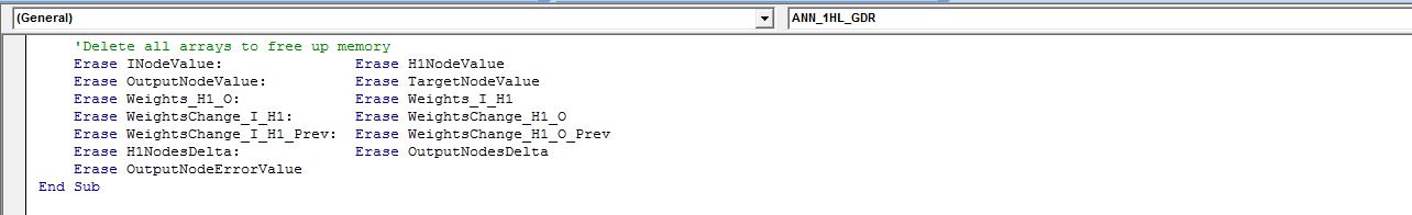
‘Delete all arrays to free up memory
Erase INodeValue:               Erase H1NodeValue
Erase OutputNodeValue:          Erase TargetNodeValue
Erase Weights_H1_O:             Erase Weights_I_H1
Erase WeightsChange_I_H1:       Erase WeightsChange_H1_O
Erase WeightsChange_I_H1_Prev:  Erase WeightsChange_H1_O_Prev
Erase H1NodesDelta:             Erase OutputNodesDelta
Erase OutputNodeErrorValue
End Sub