Today I will continue with the topic of SVM and extend the discussion to include classification problems where the data is not linearly separable.  In the previous post I described the hard margin classifier where we derived its mathematical formulation and implemented it in a spreadsheet.

Hard Margin Classifier Recap

We decided to use a hyperplane that separates our data perfectly with an additional requirement for that hyperplane to have the largest possible margin.  In case of two dimensions we can visualise this as a line separating class -1 from class +1.   Our formula for the separating hyperplane is given by wx+b=0.  Vector w is a weights vector that determines the slope of the hyperplane and the coefficient b determines the distance from the origin.  To derive the largest margin hyperplane we introduced supporting hyperplanes that were symmetrically placed on either side of the separating hyperplane and searched for vector w and b that maximized our margin delta.

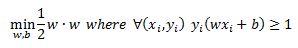
Mathematically the problem was formulated as:

We then normalized the distance between our separating and supporting hyperplanes to have a distance of 1 on either side and made some simplifications to the formulation so that the optimization can be stated as a quadratic programming problem.

The final primal optimization problem was derived to be:

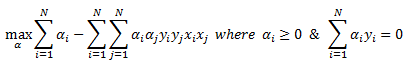
We then set up a Lagrange function and derived the dual formulation of the problem that we can pass onto the quadratic programming routine to solve for our coefficients:

Non Separable Case:

Let’s now assume that we have a dataset where the two classes cannot be linearly separated.  Most real world classification problems deal with classes that cannot be perfectly separated so this assumption is more realistic than what we dealt with earlier.  If we were to use the formulation that we derived above we would fail to find a solution because the condition y(wx+b) is equal to or greater than 1 cannot be satisfied.

To handle datasets where the classes are not linearly separable we can either use feature engineering (I will discuss this in a future post when dealing with Kernels) or we can relax the constraint that is causing us grief.

To relax the constraint that data is linearly separable we can introduce a new slack variable.  The constraint will now look like the following:

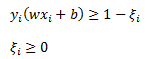
To visualize this I have added two new data points to our graph and circled them.  You can see that if we use the blue hyperplane as our classifier we would be making two errors.  The slack variables measure the extent to which the margin, y(wx+b)=1 is violated.

We can have 3 cases for any particular data point.

• Correct classification and data point does not violate the margin. In this case slack variable is equal to zero
• Correct classification but data point violates the margin. In this case slack variable is between zero and one.  This will happen when a data point is on the correct side of the separating hyperplane but is inside the margin that is defined as wx+b=1.
• Incorrect classification. This is the case that is depicted in the graph above.  The data point is on the wrong side of the separating hyperplane and y(wx+b)<0 and therefore the slack variable is greater than one.

Now that decided to introduce the slack variables we need to modify our objective function.  To balance any violations of our margin we want to penalize our objective function.  To do so we will introduce a total cost measurement.  This will capture the total number of violations we make.  I should point out that this total cost doesn’t measure the classification error rate; we are only measuring the violation of our margin.  A point can be on the wrong side of the margin but still classified correctly.  Let’s define total cost as:

We scale the sum of our slack variables by a tuning parameter C.  The value of C is not solved for in our optimization routine but is selected via cross validation.

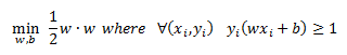
So remembering that for a linearly separable dataset our optimization problem was:

And now with the introduction of the slack variable that allows us to fit a separating hyperplane to a non separable dataset we have the following primal optimization problem:

So we are trading off total cost versus width of the margin.  Tuning parameter C controls this trade-off.  If we were to select some large value for C then we will penalize the model for any violations of the margin. In the limit as C is increased we are left with the case of a hard margin classifier.

To solve this problem we need to set up a Lagrange function which captures our amended objective function and the two constraints:

We are minimizing our objective function with respect to w, b, and the slack variable but maximizing with respect to alpha and beta.

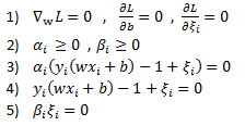
The KKT conditions for the solution are given as:

Prior to differentiating the Lagrange function lets group variables together to make things more clear

Now differentiating with respect to the vector w we only use the blue terms to get:

By setting the derivative to zero we have:

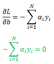
Now we differentiate with respect to coefficient b (the green term) to get and set the results equal to zero:

And finally we can take the derivative of the Lagrange function with respect to the slack variable:

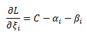
And as with the previous derivatives we set it to zero:

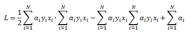
We will be using the KKT conditions and formulating the dual optimization problem to achieve some remarkable results so let’s rewrite our Lagrange as:

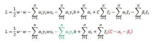
Notice that the green and red terms equal to zero at the solution due to our KKT conditions.

So we have:

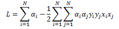
We can now substitute for the value of w what we derived from one of the KKT condition above:

And here is the very cool result; we end up with an identical set up as in the hard margin case from Part 1

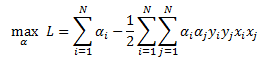
The dual problem is given by:

Subject to the following constraints:

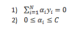
The last constraint is due to the fact that at the solution KKT condition C-alpha-beta =0 must hold.  Since alpha and beta must be equal to or greater than zero then C must be greater than or equal to alpha.

So notice what we were able to show.  We introduced slack variables to allow us to handle non-separable data but after deriving the dual formulation of the problem we are left with something that is very similar to the hard margin problem with the exception of an additional constraint that alphas must be smaller than some tuning parameter C that a user selects.

Once we use a solver to calculate our alphas we need to work out what our w vector and parameter b is to use the classifier.  Again, using KKT condition we were able to derive the value of w given alphas as:

Once we calculate vector w we can use the fact that for our support vectors (data points that have non-zero alphas) and that are not violating the margin (slack variable is equal to zero) we have:

We solve for b to get:

Once we have w and b we can use the classifier by simply plugging in some observation x and using the rule:

Excel Example:

In the workbook I set up the dual formulation of the quadratic programming optimization.  We are trying to maximize cell D4 by changing values of alpha.  Once we solve for aphas we can calculate w and b in cell M2:M4.  With our coefficients in hand we can assign a class label to a new data point in cells P4 and Q4.  We can control the cost parameter C in cell D3. svm_calcs_example

Sanity Check:

As in Part 1 we can run a quick check to make sure our implementation matches R.

Our results match so we can have some confidence that our spreadsheet is set up correctly.

Hope you enjoyed.

Some Useful Resources:

• Idiot’s Guide to SVM from MIT http://web.mit.edu/6.034/wwwbob/svm-notes-long-08.pdf
• Andrew Ng notes http://cs229.stanford.edu/notes/cs229-notes3.pdf
• Lecture 15 on Kernel Methods from Yaser Abu-Mostafa at Caltech https://work.caltech.edu/telecourse.html
• Christopher Burges “A Tutorial on Support Vector Machines for Pattern Recognition” http://research.microsoft.com/pubs/67119/svmtutorial.pdf
• Practical Mathematical Optimization by Jan A Snyman is excellent http://www.springer.com/us/book/9780387243481