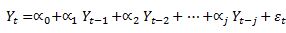
Granger causality is a simple formulation to test if preceding values of a variable X help explain some of the variance observed in variable Y. To test for this we first need to regress Y on past value of itself to capture any autoregressive features. Typical set up of the test sets up below equation:

Users will select the number of lags often with the help of BIC or AIC information criterion.

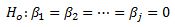
Granger causality test is a test of a joint hypothesis that lagged values of X are not statistically significant. Therefore the null hypothesis is:

While the alternative hypothesis:

To test the null hypothesis we need to estimate two models. One is a restricted model which omits historical values of X

This is a restricted model while the second model has the full specification that we mentioned above:

To test for Granger causality we need to carry out an F-test which compares the Sum of Squared Error from the restricted model (SSE_r) with the Sum of Squared Errors of the unrestricted model (SSE_u). If SSE_u is statistically different from SSE_r then the restriction of omitting past values of X is not valid. The F-statistic is given by:

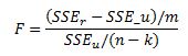
where m is the number of restrictions. In our case this will be the number of lagged X values that we have omitted from the unrestricted regression. n is the number of observations in our historical sample. k is the total number of parameters estimated in the unrestricted model (constant included).

Once we have the F-statistic we can compare it to a critical value to see if we can reject the null hypothesis of X not Granger causing Y.

The above procedure is usually done for both time series to see if X->Y (notation for X Granger causing Y) and also to see if Y->X (Y Granger causing X). After carrying out these tests we can have following outcomes:

1) Unidirectional causality X->Y but not Y->X

2) Unidirectional causality Y->X but not X->Y

3) Dual causality where X->Y and Y->X

4) No Granger causality

To carry out this procedure in excel we will test to see if weekly change in EURUSD 1month 25d risk reversal is Granger caused by weekly changes in spot FX rate. We will also test the causality the other way where we test to see if changes in 25d risk reversal Granger causes changes in the spot exchange rate. Our data sample goes back 4 years.

First we load the data and set up a column for each lag. Our first test is to check if spot changes Granger causes changes in the risk reversal. We will run the test using 2 period lags. The unrestricted equation becomes:

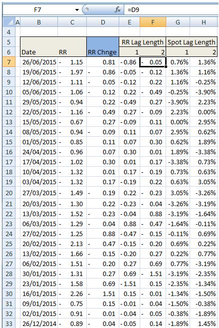
We can use LINEST(D7:D238,E7:H238,TRUE,TRUE) in excel to estimate the regression model and get the SS_u value.

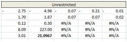
The bold value is the model’s sum of squared errors

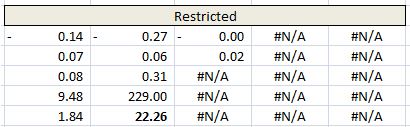
We need to repeat the process and estimate the restricted model as:

This is again done with the LINEST(D7:D238,E7:F238,TRUE,TRUE) function but now inputting only the column ranges that contain lagged RR data.

The output looks like below

Now we can compute the F-statistic. Note that in our case we have 232 weekly observations that are included in the model. Therefore n = 232. k is equal to 5 since that is the number of parameters we estimated in the unrestricted model. We removed 2 parameters to estimate the restricted model so that is the value we should use for m. Therefore F = ((22.261-21.0967)/2)/(21.0967/(232-5))= 6.264. Once we have the F-statistic we can use excel’s FDIST function to calculate the p-value using m and n-k as the degrees of freedom. in our case =FDIST(6.264,2,232-5) which equals .22%. Since this value is below 1% then we can say that we reject the null hypothesis of no Granger causality from spot changes to RR changes at 99% confidence level.

Notice that we didn’t report the estimated coefficients. We are only interested to test for Granger causality instead of looking at the structure of the full model and the estimated coefficients.

We can now repeat the same exercise but now with below unrestricted model:

Noting the SSE_u and moving on to estimate the restricted model

And again noting the SSE_r and calculating the F statistic and p-value.

In our case we have:

Therefore we can conclude that changes in spot FX rate Granger cause changes in the 1 month risk reversal but changes in the risk reversal do not Granger cause changes in spot.

This was a post to show a simple example of Granger causality testing in excel. We will have more to say on Granger causality and also a more systematic look at risk reversals in FX in upcoming posts.

Some useful resources:

Wikipedia entry for Granger Causality: https://en.wikipedia.org/wiki/Granger_causality

Excellent book on econometrics: http://www.amazon.com/Basic-Econometrics-Damodar-Gujarati/dp/0073375772/ref=sr_1_1?s=books&ie=UTF8&qid=1435312941&sr=1-1

Another handy book on econometrics: http://www.amazon.com/Analysis-Financial-Data-Gary-Koop/dp/0470013214/ref=sr_1_4?s=books&ie=UTF8&qid=1435313038&sr=1-4&keywords=gary+koop+data