In our previous post we showed a simplistic implementation of a logistic regression model in excel. In practice we need to be able to estimate a multivariate version of the model and also asses the quality of the model calibration. All the requirements make a spreadsheet implementation impractical and we need to rely on VBA.

We relied heavily on four sources that are listed at the end of the post.

The VBA code that is provided at the end of the post implements Newton’s method to maximize the log likelihood function with respect to beta parameters based on supplied factors. The function works similar to Excel’s native LINEST function.

Function name is Logit and needs to be entered as an array function with Ctrl+Shift+Enter after the arguments of the model are input:

Function Inputs

Known_y: This is our list of 0s and 1s. We input a 1 for a positive instance of the binary variable that we are trying to mode. The data series should be entered in a single column. In our previous post y = 1 if a recession started 3 months in the future from the observation date and zero otherwise.

Known_x: This is a list of our explanatory variables. These can be continuous or discontinuous (dummy) variables. In the previous post we had a single independent variable to forecast recessions which was the yield curve slope.

Cutoff: This is a user supplied probability that will mark the demarcation between a positive and negative instance that we assign to our model output. For example a probability of .5 is assigned as a cut-off and therefore if our model estimates a probability of .5 or higher we assume that our forecast for y is 1. This value should be bounded between 0 and 1. Different variants of the cut off can be used when assessing the quality of the fitted model. The use of this cut off value will become clear when we discuss contingency tables.

Constant: The default settings is TRUE. When TRUE is selected the model will be built with a constant (there is no reason not to have a constant in the model)

Stats: the default setting if the argument is omitted is FALSE. When the argument is omitted or is set to FALSE, only the beta coefficients are reported. If TRUE is selected, multiple statistical tests are reported.

Function Outputs

Rows

1)  Data Labels

2)  Estimated Coefficients

3)  Standard Errors of the estimated coefficients which is equal to negative of the square root of the diagonal value of the Hessian matrix

4)  z-score of the estimated beta coefficient. It is equal to

5)  p-value of the test statistic using standard normal distribution. It is the probability of the coefficient being equal to zero

6)  MacFadden pseudo R²

7)  Cox and Snell pseudo R²

8)  Number of iterations needed to reach the maximum of the log likelihood function

9)  The likelihood ratio test statistic

10)  p-value of the likelihood ratio statistic

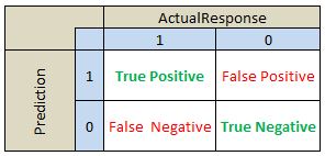
The rest of the output is based on classification ratios. The second block contains a contingency table. To interpret the results lets define the following values:

True Positive: Number of observations predicted to be 1 (ie estimated probability from the model is greater than our selected cut off value) and actual observed value is 1.

True Negative: Number of observations predicted to be 0 (ie estimated probability from the model is less than our selected cut off value) and actual observed value is 0.

False Positive: Number of observations predicted to be 1 (ie estimated probability from the model is greater than our selected cut off value) and actual observed value is 0. This is a prediction error.

False Negative: Number of observations predicted to be 0 (ie estimated probability from the model is less than our selected cut off value) and actual observed value is 1. This is a prediction error.

The reported contingency table is organized as outlined below:

To help with the analysis of the quality of the classification/prediction model we report below ratios in the final block of the output of our function:

Accuracy: Number of correctly predicted instances as a ratio of total number of observations

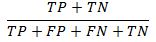
ErrorRate: Misclassification or prediction errors. this is 1- Accuracy

HitRate: This is number of successful predictions of 1s versus all instances of 1s

TrueNegRate: This is the number of times that we correctly predict 0 as a ratio to all observations where y is equal to 0

FalsePos: The number of times the model incorrectly predicted 1 as a ratio of all instances of 0

Precision: Number of correctly predicted 1s divided by the total number of predicted 1s

NegPredVal: Total number of correctly predicted 0s divided by the number of 0 predictions

FalseDiscover: This is the number of times the model incorrectly predicted 1 divided by the number actual number of 1s

The code is presented below:

This block of code loads in the data and declares arrays needed to hold the data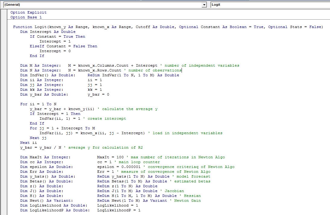

The second block of code implements Newton method to estimate the beta coefficients

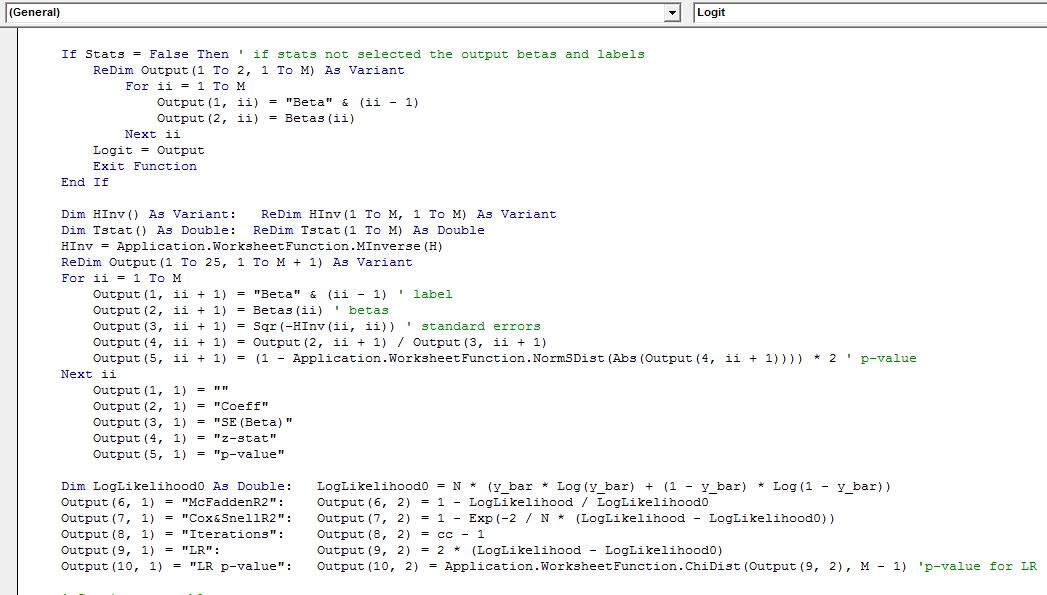
Here we calculate the Goodness-of-Fit statistics

The final block of code below calculates the contingency table and classification statistics and some code to tidy up the output so that its more presentable and easy to read.

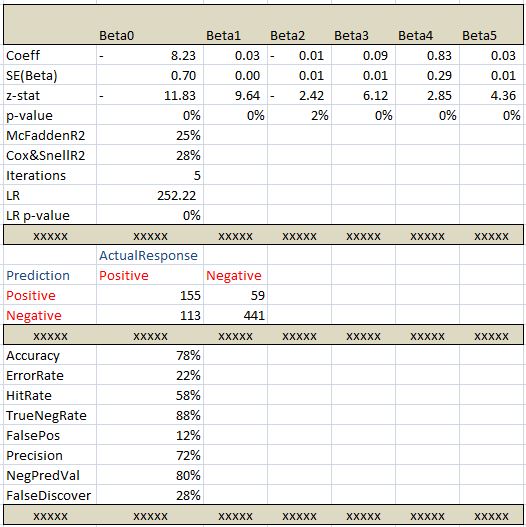
Below is what the output looks like after some formatting to make the tables easier to read. This is an output of the single call of the function. When calculating statistics make sure you select 25 rows and the number of columns should equal the number of beta parameters you are estimating plus one additional column for labels.

Binary response models are widely used. Below is a small list of examples of how they can be used in finance:

1. Currency crises prediction
2. Carry trade unwind
3. Recession prediction
4. Equity excess return prediction
5. Corporate takeover targets
6. Central bank monetary policy changes

Some useful resources:

1) Making Sense of Data II by G Myatt and W Johnson: http://as.wiley.com/WileyCDA/WileyTitle/productCd-0470222808.html

2) A Guide to Modern Econometrics by M Verbeek: http://as.wiley.com/WileyCDA/WileyTitle/productCd-EHEP002634.html

3) Credit Risk Modeling using Excel and VBA by G Loffler and P Posch: http://as.wiley.com/WileyCDA/WileyTitle/productCd-0470660929.html

4) Logistic Regression: a primer by F Pampel: http://www.sagepub.com/textbooks/Book10146