I am back after a two week trip to the land of twisted melodramatic tv series, androgynous boy bands, delicious food, and perennial jingoistic posturing by a divided people. I am obviously talking about Korea. Was such a pleasure to visit with family and bounce around Seoul. Now it’s time to catch up with the markets. Today’s post will be short and will present a very useful interpolation method that is commonly used in the industry but is hardly mentioned in finance literature. The interpolation method is called Akima spline and is named after the author.

Most often discussed spline method is the cubic spline.   Implementation in VBA is given in Option Pricing Models and Volatility using Excel-VBA by Fabrice Rouah and Gregory Vainberg. A well known issue with a cubic spline is that it is not local. This means that if there is an outlier in the data set then the curve around surrounding points is “wobbly”. Akima spline is much more stable and is not influenced by outliers to the same extent. Below is a visual example of this point given in The Computer Graphics Manual by David Salomon.

What Akima suggested in his 1970 paper was to fit a cubic polynomial between two points x(i) and x(i+1).

Two constraints on the polynomial is that the function to the left of x(i) produces the same y value as the function to the right of x(i). Similar continuity constraint is imposed at x(i+1). In addition, Akima also imposed at each point x(i) a constraint that the slope t at point x(i) is equal to:

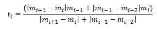
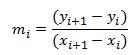
where each m is a straight line between surrounding segments of the curve (secant), and is defined as:

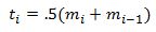
In a special case where the denominator in the formula for t is equal to zero we instead will use:

This is very easy to implement in VBA but one point should probably become apparent now. How can we fit a cubic polynomial that starts from the left most point and ends at the right most point if we do not have enough information to compute the secants beyond those data points. Akima suggested extrapolating the data by assuming that 2 points to the left and two points to the right of our data lie on a quadratic function defined as:

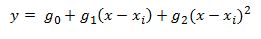
where all g’s are constant. This yields (assuming end point is x3):

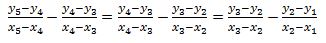
This of course implies that we can compute the extrapolated secants preceding our first x value as:

and we can compute the extrapolated secants beyond our last data point as:

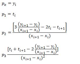
Now we have enough information to derive the coefficients of the interpolating cubic polynomial between any pair of our given data. The final formula is given by:

where:

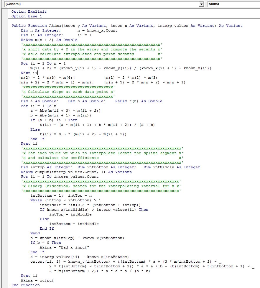
Below is the VBA function

As a check we run R’s aspline as a check against our implementation:

The results appear to match exactly.

Some Useful Resources:

1) Akima’s paper http://www.leg.ufpr.br/lib/exe/fetch.php/wiki:internas:biblioteca:akima.pdf

2) The computer Graphics Manual by David Salomon http://www.springer.com/us/book/9780857298850 (discussion of Akima spline is available on Google books)

3) Matlab implementation by Joe Henning http://www.mathworks.com/matlabcentral/fileexchange/36800-interpolationutilities/content/cakima.m

4) R akima package description https://cran.r-project.org/web/packages/akima/akima.pdf