Today will be a quick post that is part of a series on FX volatility skew in G10. To do that we will have a look at implied versus realised skew. To decompose realised and implied skew we will use the following definitions.

Implied Skew is the change in implied volatility that is priced into today’s surface assuming perfect foresight by the market of what the FX return is going to be in the future. That is, at time t = 0 we can check what the implied volatility is of a strike that is the actual at the money strike at some future date t = T.   For example, on 14Sep2015 the AUDUSD 3 month volatility smile looked like below:

On 14Sep the atm volatility was 12.95%. A week later, on 21Sep, the 3 month ATM strike was .7130. Using the smile as of 14Sep we can check what the implied volatility was of the .7130 strike to assess what was the implied skew. In this case the .7130 strike had an implied volatility of 12.85%. Taking the difference between the two we get -.10% [12.85-12.95]. Therefore what we will call implied skew is the difference between the implied volatility of the ATM strike that is observed on 14Sep and the implied volatility on 14Sep of what is the actual atm strike a week later on 21Sep.

Remember the point of this is simply to see what the 14Sep surface was pricing in terms of the dynamics of the implied volatility assuming perfect foresight by the market of what the atm strike would be in the future. This may not seem relevant here but what we would like to check is if there is any systematic deviation from the implied skew and realised skew. Now in our case we can check to see what the 3mth smile actually looks like on 21Sep.

The actual ATM implied vol on 21Sep is 12.50%. Therefore the fixed strike volatility change for the 21Sep atm strike of .7130 is the difference in vol of the .7130 strike from 14th to 21st of Sep. In our example it is -.35% [12.50-12.85]. We can combine the two effects, implied skew and fixed strike vol change, to define realised skew. In our case it is -.45% [12.5-12.95] which is the total change in the implied volatility from the 14Sep atm strike to 21Sep atm strike.

and

These definitions may seem confusing so hopefully the graph below will help to clarify the concepts.

The blue curve is the 3month AUDUSD smile as of 14Sep and the grey curve is the 3month AUDUSD smile as of 21Sep. What we defined as the implied skew is the difference between the volatility marked with the green and red parallel lines. A way to think of it is that if we bought the .7130 strike option on 14Sep at vol of 12.85, which is at a .05vols discount to the atm, we would find ourselves holding a atm option on 21Sep. If the new atm vol on 21Sep is different from 12.85 we would have vega PnL. We are ignoring delta, theta, gamma, vol slide (and other higher greeks) PnL here. Now on 21Sep the actual atm volatility is 12.50. This is the blue parallel line that touches the grey smile curve. We can decompose that into the fixed strike change (curly red bracket) the implied smile (curly green bracket) which gives us realised skew (the blue curly bracket).

Now for an explanation for why we are going through the trouble. We want to see if on average the implied skew is less than or greater than the realised skew. We want to see if the implied skew is close to actual changes in implied volatility on average.

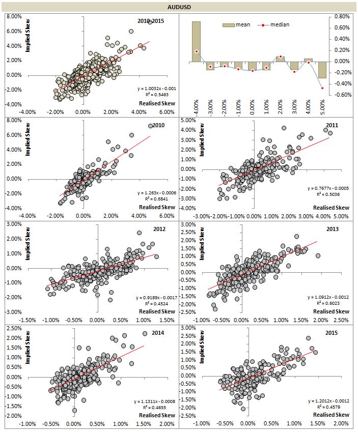
To do this we will look at realised skew versus implied skew. Realised skew is measured over a one week holding period. We will take overlapping daily observations. For example for AUDUSD we can construct a scatter plot and run regression between the two variables. Below are the results for the period covering 2010 to Sep 2015:

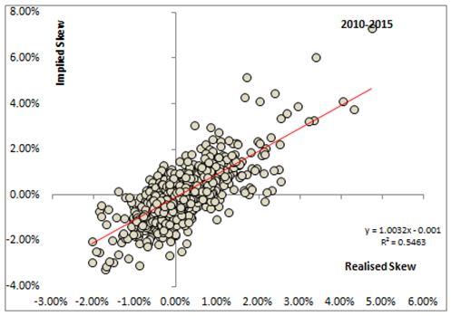
We can see that on average realised skew has a one-to-one relationship with implied skew (beta is lose to 1). If beta is greater than one that means implied skew is larger than realised skew and if beta is less than 1 that implies that realised skew outperforms implied skew.

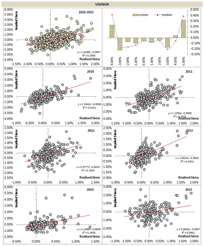
To check if realised and implied skew has different behaviour depending on the change in the underlying we can split the data into ranges of weekly atm strike change and then look at what realised skew minus implied skew was on average for each bucket. For AUDUSD we have:

What the graph reveals is that for small changes in the underlying realised skew underperforms implied skew. It is only for outsized moves to the downside when realised skew outperforms implied skew. We include average and median as measures to highlight possible outliers. In case of AUDUSD weekly changes of 4% or more we see that the average realised skew outperformance is significant but the median is much lower, implying that there have been some instances where realised skew significantly outperformed implied skew to bring the average up above the median.

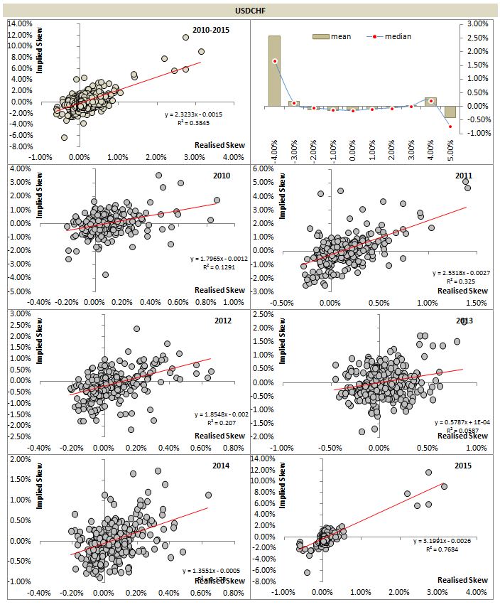
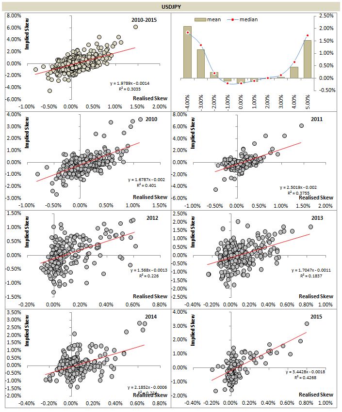
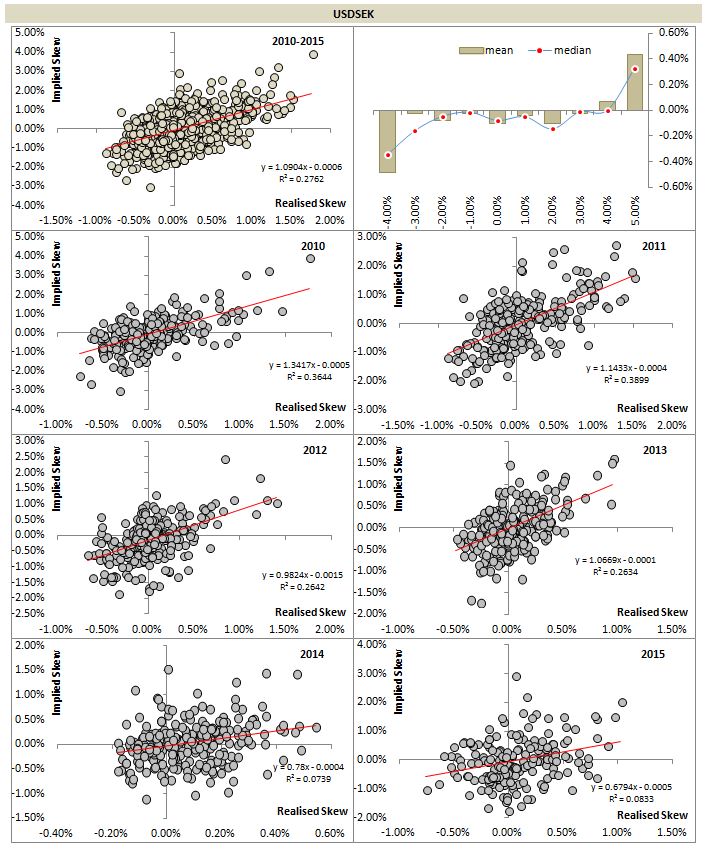
We can further disaggregate the data based on year to check for stability of the relationship. Below are the full results for G10: