With the disappointing Nonfarm Payrolls print this Friday I decided to have a systematic look at how well common machine learning algorithms can nowcast this particular series.

Dataset Description

• Private Nonfarm Payrolls. The most important statistic in the market and generates the most volatility.  Released on first Friday of a month and measures the monthly change in the number of employees on business payrolls. This is the target variable in the models.  I also include lagged values to capture autocorrelation.
• Temporary Help Services. This statistic is released on the same day as the Nonfarm payrolls data and captures shifts in hiring of temporary workers.  Increase in temp hiring is potentially a leading indicator for the labour market and is lagged in my models. I use up to 3 historical monthly readings.
• ADP Private Nonfarm. Automatic Data Processing Inc is a leading payroll related services provider. Data from 3650 of their private clients is used to construct a forecast of the official NFP release.  The model used to generate the NFP forecast is built in collaboration with Moody’s Analytics.  This is a timely report since it precedes NFP by two days.
• Initial Claims 4 week average. A moving average of the weekly initial unemployment claims.
• Continuing Claims MoM change. Monthly change in the number of people that have filed jobless claims with the appropriate government labour office.
• Manufacturing PMI Employment Index. A diffusion index of a monthly survey by ISM of supply management professionals.  Readings above 50 means factories are hiring new workers.
• Non-Manufacturing PMI Employment Index. Similar to the manufacturing index but surveys the service industry.
• Conference Board Labour Differential Index. This is a report that surveys approximately 3000 households about their confidence about the labour market.

Model List:

Below is a sample list of some popular regression modeling approaches in machine learning which I will consider.  R’s caret package has a function train that can handle all these models and much more.  More on this package at http://topepo.github.io/caret/

• Ridge Regression [100 models].   
  • Tuning parameter: Labda
• Support Vector Regression with Linear Kernel [100 models].
  • Tuning parameter: Cost
• Support Vector Regression with Polynomial Kernel [400 models].
  • Tuning parameter: Polynomial Degree, Cost, Scale
• Support Vector Regression with Radial Basis Function Kernel [500 models].
  • Tuning parameter: Cost, Sigma
• Stochastic Gradient Boosted Trees [684 models]
  • Tuning parameter: Number of trees, Maximum depth of tree, Shrinkage
• Cubist [36 models]
  • Tuning parameter: Number of trees, Maximum depth of tree, Shrinkage
• Neural Network [50 models]
  • Tuning parameter: Number of nodes in a hidden layer, Weight decay
• Nearest Neighbor Method [30 models]
  • Tuning parameter: number of clusters

In total I will consider 1900 models. For each class of models repeated 10-fold cross validation will be performed with 5 repeats to select optimal tuning parameters.  Fifty monthly observations will be left out for testing model performance.  In total I have 131 monthly observations for the period starting Jun 2005 and ending Apr 2016.

my.data<-read.csv('nfp2.csv')
(n<-nrow(my.data))

train.data<-my.data[51:nrow(my.data),] # data for model tuning
test.data<-my.data[1:50,] # data for model generalization

require(caret) # caret package for train function
train.cntrl<-trainControl(method = 'repeatedcv', number = 10, repeats = 5)

 

In today’s blog I will present the R code for Ridge Regression, SVM with linear and polynomial kernel.  Caret’s github page has the details about all other models and readers should be able to easily replicate my results.

Ridge Regression Results:

We can estimate the model using below code

####################################
# Ridge Regression Model
####################################
set.seed(81)

ridge.grid<- data.frame(.lambda = 10^seq(1, -5, length = 100))

ridge.fit<-train(train.data$NonFarm~.,
data=train.data,
method='ridge',
tuneGrid=ridge.grid,
trControl=train.cntrl,
preProc =c('center','scale'))

plot(ridge.fit) # plot CV profile
ridge.fit$results[ridge.fit$bestTune[[1]]==ridge.fit$results[,1],] # return RMSE for optimal lambda

ridge.test.predict<-predict(ridge.fit, newdata=test.data) # test data fit
(ridge.test.rmse<-sqrt(sum((test.data$NonFarm - ridge.test.predict)^2)/nrow(test.data))) # test RMSE

 

The cross validation RMSE vs lambda parameter profile is presented below:

The optimal lambda parameter of .0142 results in RMSE of 75.56 and Rsquared of 84%.

SVM- Linear Kernel Results:

To estimate Support Vector Regression model with a linear kernel we can use below code:

####################################
# svm linear kernel
####################################

set.seed(81)

svm.linear.grid<- data.frame(.C = 1:100)

svm.linear.fit<- train(train.data$NonFarm~.,
data=train.data,
method = 'svmLinear',
trControl = train.cntrl,
tuneGrid=svm.linear.grid,
preProc =c('center','scale'))

The cross validation plot is below:

The optimal cost parameter of 1 results in RMSE of 74.95 and Rsquared of 85%.

SVM- Polynomial Kernel Results:

To estimate SVM with polynomial kernel we set up a grid of tuning parameters and use the train function as in previous examples.

####################################
# svm polynomial kernel
####################################

set.seed(81)

svm.poly.grid<- expand.grid(.degree =c(2,3),
.scale=10^seq(2, -5, length = 20),
.C = 2^seq(-2, 7, 1))

 

CV RMSE profile:

The optimal model has degree of 3, scale of .0002976, and a C value of 128. The reported RMSE is 74.74 and R squared of 85%

SVM- Radial Basis Function Kernel Results:

With radial basis kernel we have two tuning parameters

####################################
# svm radial basis
####################################

set.seed(81)

svm.rbasis.grid<- expand.grid(.C = 2^seq(-2, 7, 1),
.sigma=seq(1 , 50, by=1 )/100)

The optimal cost parameter is 8 and vol of .01.  Best RMSE is 75.13 and Rsquared is 85%

Boosted Trees Results:

Gradient Boosting Machines are all the rage so lets see how they fit our data.  We can use the gbm package in R. Lets set up a tuning grid and check cross validation RMSE.

####################################
# gbm
####################################

set.seed(81)

gbm.grid<- expand.grid(.interaction.depth = seq(1, 7, by = 2),
.n.trees = seq(100, 1000, by = 50),
.shrinkage = c(0.01, .05, 0.1),
.n.minobsinnode=c(5,10,20))

Optimal tuning values for the model were 550 trees with a depth of 1, a shrinkage parameter of .01. and minimum number of observations in a node of 5.  RMSE is 83 and Rsquared if 82%.

Cubist Results:

Optimal tuning values of 0 neighbors and 5 commitees returned RMSE of 76.98 and Rsquared of 84%.

####################################
# cubist
####################################
set.seed(81)

cubist.grid<- expand.grid(.committees = c(1, 5, 10, 50, 75, 100),
.neighbors = c(0, 1, 3, 5, 7, 9))

Neural Network Results:

A neural network with a single hidden unit and weight decay of .25 resulted in RMSE of 91 and Rsquared of 79%

####################################
# nnet
####################################
set.seed(81)

nnet.grid<- expand.grid(.decay = c(0.01, .05, .1, .25, .5),
.size = 1:10)

Nearest Neighbor Results:

This is the last model that I fitted.  The optimal number of clusters was 6 which resulted in a cross validation RMSE estimate of 88.9 and Rsquared of 78%.

####################################
# knn
####################################
set.seed(81)

knn.grid<- data.frame(.k = 1:30)

Model Comparison:

We can also perform inter model comparison in R.  Because we used the same repeated cross validation specification for all the models and we set the same seed prior to training we have paired samples ready for comparison.  With 10-fold cross validation and 5 repeats we have 50 resamples for each model.  We can use caret’s resamples and diff.resamples functions to check if the difference in model  performance metrics are statistically significant.

#######################################
# Check model diff
#######################################
resmpl <- resamples(list(Ridge = ridge.fit,
SVM_lin = svm.linear.fit,
SVM_poly=svm.poly.fit,
SVM_rbf=svm.rbasis.fit,
GBM=gbm.fit,
Cubist=cubist.fit,
NeuralNet=nnet.fit,
KNN=knn.fit))

model.diff<-diff(resmpl)
summary(model.diff)

I exported the data into excel and formatted the table for easy comparison.

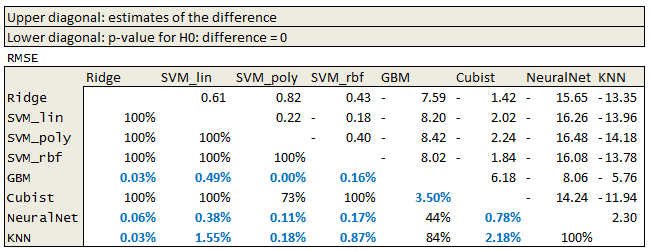
The results suggest that GBM, Neural Network and k-nearest neighbor methods are inferior.

Finally, we can check how well the models generalize by checking RMSE on our test data.  Below is a table with the first 6 columns reporting summary statistics of the RMSE metric that we obtained on the cross validation run.  The last column reports the RMSE on our test data. Unsurprisingly the cross validation RMSE is more optimistic than the test data RMSE.  Since I used data from Apr 2001 to May 2005 as the test data there is some hope that this is the upper bound on the true RMSE.  This is possible since the test data is older and we used more recent (perhaps more relevant) data in the model calibration.

Models vs Market:

This was a simple exercise in model selection and it produced modest results.  We live in a data rich world and I used a minuscule number of features compared to the data that is available.  I omitted regional labour market indexes like Empire State Manufacturing Index, PhillyFed Index, all of the detailed data that is released by BLS as part of its employment report.  Non conventional sources of data can also be included for consideration.  Google trend data on key search terms is one example.

Having said all that it is time to check how the models compare to the market consensus estimate for Nonfarm Payrolls.  Since Jun 2005 to present the RMSE of the bloomberg consensus estimate has been 62k!  This reveals that the market forecast is based on a much more rich information set than the one considered here.

Useful Resources:

• I have mentioned this in many posts, Applied Predictive Modeling is a MUST. All of the models I mentioned in this post are in that book and MUCH MUCH MUCH more http://appliedpredictivemodeling.com/
• Caret github page https://topepo.github.io/caret/
• Slides on Cubist model https://cran.r-project.org/web/packages/Cubist/vignettes/cubist.pdf
• Good book on economic data releases https://www.amazon.ca/Secrets-Economic-Indicators-Investment-Opportunities/dp/0132932075