Haven’t had the time to add posts recently due to traveling plans but I’m back for a week and have sketched out a plan for a series of posts on predictive modeling.  I recently received a fantastic bday present in the form of Applied Predictive Modeling by Max Kuhn and Kjell Johnson and highly recommended it for R enthusiasts.

Today I want to tackle a section out of the Linear Regression and Its Cousins chapter. I’m talking about Ridge Regression.  At the core of Machine Learning/Data Mining/Statistical Learning is the concept of bias/variance trade off.  Wikipedia has a good entry on the topic and I provide a link below.

In linear models space the trusted Ordinary Least Squares (OLS) model is the best linear unbiased estimator (BLUE) when certain conditions are met. More often than not these assumed conditions are not satisfied and therefore we can improve on the OLS model, in the sense of smaller mean standard error (MSE).  For prediction purposes we can select a model that is slightly biased but in exchange for the increase in bias we can reduce the variance of the model significantly.  One of the ways to perform this trade off is with the Ridge Regression model.

Exposition and Derivation:

Before deriving the Ridge Regression model it is probably helpful to remind the reader how the OLS parameters are defined and estimated and then contrast it with Ridge Regression.  In the case of OLS we first set up a cost function which penalizes us for estimation error.

Visually we are trying to fit a straight line that minimizes the sum of the squares of the vertical distances from the regression line to the observation points.  The reason why we chose the squares is to control for under/over prediction and also to penalize large errors more than small errors. * Note that the image was taken from another excellent book by Gareth James, Daniela Witten, Trevor Hastie and Rob Tibshiran called Introduction to Statistical Learning

The linear model can be written as:

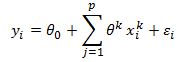
where y is the observation of the true data point, each x is our independent variable, the thetas are the coefficients that we are trying to estimate and epsilon is our forecast error.  In our example there are p independent variables and a total of n observations.  So in total we will have n equations for each observation.  We can write out this system of equations in matrix form as:

Here we simply set x  indexed at k equal to zero to 1 which will yield the intercept term.  We now have y and e as nx1 column vectors, theta is a (p+1)x1 column vector and X is an nx(p+1) matrix.  The error vector is equal to:

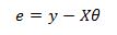
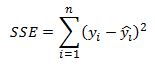
Our cost function (sum of squared residuals) can be written compactly as:

Here the dot product of the residuals produces the sum of squared residuals that we are after.  It is this quantity that we wish to minimize with respect to the theta coefficients. To proceed we will expand the right-hand side of the above equation:

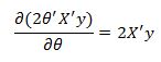
Now to minimize this function with respect to our theta coefficients we need to take the derivative of this function and set it equal to zero and solve for theta.

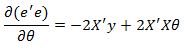
The first part of the function does not depend on theta so its derivative with respect to theta is zero.  The second part of the equation has a derivative equal to

Also, the derivative of the final term is equal to

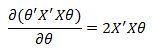
Putting this together we have:

Setting the derivative to zero and solving for theta we get:

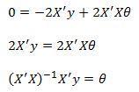
These are the famous Normal Equations for the least squares regression that produce the theta coefficients.

In instances when there is high correlation among the independent variables (features) we often observe large absolute values of the coefficients.  This is where Ridge Regression comes in.  We will introduce a penalty for large coefficients into our cost function.  This will also help deal with cases when we are over fitting our data.

Recall that the cost function was given as the sum of squared residuals:

in vector form this is

We now introduce an additional term to the equation:

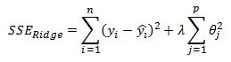
Here lambda is a shrink factor that is determined outside of the model (ie it is a tuning parameter) and it assigns a weight to how much we wish to penalize the sum of squared coefficients.  When lambda is equal to 0 we revert back to the OLS model.  When lambda increases to infinity all the parameters are set to zero.  Also, and this is an important point, when we increase the lambda parameter we are increasing the bias of the model but reducing the variance. Alternatively, when we reduce lambda we are reducing the bias of the model but increasing the variance. We can search for a lambda value that produces an ‘optimal’ trade off between bias and variance that hopefully generalizes well and will produce superior predictive performance compared to OLS.

I should also mention that Ridge regression is closely related to the LASSO model where the only difference is that the penalty terms takes the sum of absolute values of the coefficients instead of their squares.  So in LASSO we have:

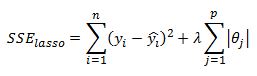
The LASSO model has some very desirable properties such as feature selection. This means that as one increases the lambda parameter some of the thetas are set to zero.  In case of Ridge Regression the parameters are forced to zero but do not equal zero. The result is that in the case of LASSO we get a spars solution set with few features but with Ridge we keep almost all of the features but with many close to zero.  The benefit of Ridge Regression is that is has a closed form solution similar to OLS, but LASSO does not and we need to rely on numerical minimization routines to solve for the parameters.

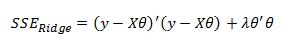
This now leads us into how can we solve for the Ridge Regression parameters.  To begin lets write the cost function in matrix form as:

We already derived the derivative of the first terms so we will proceed directly to the penalty term to get:

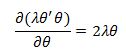
Recall that we previously had the result:

So we are left with:

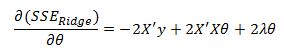
Setting this to zero we have:

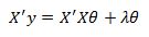
Also, lets multiply the last term by the Identity matrix I so that we can factor out the theta vector. This does not change the result since by definition a matrix multiplied by the Identity matrix is equal to itself. After introducing the identity matrix and little algebra we get:

And this is our solution for the theta coefficients given a parameter lambda.

Important Omissions So Far:

Some important issues that I left out so far is that it doesn’t make a lot of sense to penalize the intercept term.  One way to handle this is to modify our identity matrix by setting the first entry to zero.  This approach works because the first column of our X matrix are all set to ones in order to set the first theta coefficient to the intercept term.  Also, when the independent variables are on different scales there is distortion in our penalized coefficient estimates because we are penalizing them equally.  For example, if in our model we are trying to estimate the price of a house as a function of the lot size and number of bedrooms, the scale of the two variables is large and hence the size of the coefficients should be very different.  It is important to normalize the data prior to estimation of the coefficients so that they are all on the same scale.  Typical normalization procedure is to subtract the means of the feature from each observation of that feature and divide by its standard deviation.  A final point that is important, is that  in all software implementation of Ridge Regression (and OLS for that matter) the inverse of a matrix is never taken because it is computationally intensive.  More efficient numerical techniques are used to solve for the model coefficients.  But for my purpose taking an inverse works just fine so I continue to use it when working in excel.

Worked Example:

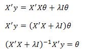
To show you first excel implementation I retrieved the Hitters dataset from R’s ISLR package.  Below is the raw data with a column of ones added for the intercept term. In total there are 20 features (including the intercept).

We then need to normalise the data by subtracting the mean of each feature and its standard deviation.  Below is a screenshot

We name the range where we have our features X, and the target variable Salary we name Y.

Now we need to create a matrix where the main diagonal has values of lambda on its main diagonal and zero elsewhere.  Since we are including an intercept term in the model we set the first entry in this matrix to zero.  We then call this range IL.  Once again the screenshot is below

Important to note that we arbitrarily selected a value for lambda of 100 at this point.

We now have everything we need to calculate the Ridge Regression coefficients.  We simply use our derived close form solution and input it as an array function.  You can see the formula in the formula bar in the screenshot.

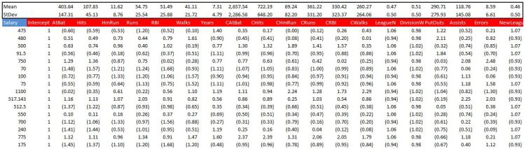
I’ve also set up a table that looks at a grid of different lambda values to see how the coefficients evolve.  As we already discussed, as lambda increases we are penalizing the model by increasing the cost function and therefore forcing our coefficients to zero.

A common way to see this dynamic is by plotting each coefficient as a function of lambda.  From below we can see how coefficients are moving towards zero as we increase lambda.  When Lambda is zero we simply have the usual OLS estimate.

Final Points

This is pretty much all there is to implementing Ridge Regression.  Hopefully this whetted your appetite to learn more. I will follow up with a post on penalized regression in upcoming days, when discussing markets and how these models can be adapted.  I wanted to leave you with a method of how lambda is usually ‘optimized’ in practice.  The approach usually involves use of some form of cross-validation.  Most common method is using K-fold validation.  This approach requires you to select a grid of possible lambda parameters.  Then, for each value of lambda you partition your data into K equal-ish parts and hold out one part from the model and then estimate the coefficients and calculate the sum of squared errors on the data that was left out.  You then move on to the second fold and strip that our of your dataset while returning the first fold.  You again estimate the model parameters and calculate the sum of squared residuals, but this time on the second fold. This is repeated K times for a particular value of lambda.  You then take an average of your K sums of squared errors to estimate the cross-validation error.  This process is repeated for each lambda value in your grid and you select that lambda value which produces the smallest cross-validation error.  In R glmnet package produces such a plot and the user typically selects the lambda that produces the smallest SSE. An example of such a plot is below.

VBA Implementation:

The first function creates a diagonal vector of lambda.

Excel has native function for matrix transpose, multiplication and inverse but unfortunately there is no function for matrix addition so we need to implement it ourselves. Below is the code

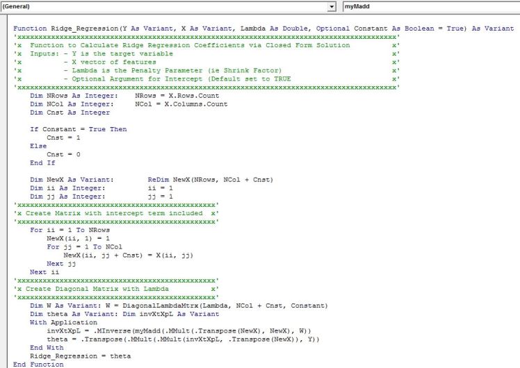
Finally, below is the main function for Ridge Regression.  It needs to be input as an array function by pressing Ctrl+Shift+Enter. A row vector of coefficients is returned and is ordered just as our matrix X.  Remember to select a range that has one row and the number of columns should equal the number of features in your model plus one for the intercept.

Some Useful Resources:

1) Note deriving normal equations http://www.stat.wisc.edu/courses/st333-larget/matrix.pdf

2) Wikipedia entry on bias variance trade off https://en.wikipedia.org/wiki/Bias%E2%80%93variance_tradeoff

3) OLS assumptions https://en.wikipedia.org/wiki/Ordinary_least_squares#Assumptions.

4) Fantastic book on predictive modeling http://appliedpredictivemodeling.com/

5) Excellent book that is free on statistical learning http://www-bcf.usc.edu/~gareth/ISL/data.html