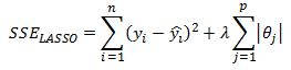
Previously I discussed the benefit of using Ridge regression and showed how to implement it in Excel. In this post I want to present the LASSO model which stands for Least Absolute Shrinkage and Selection Operator. We are again trying to penalize the size of the coefficients just as we did with ridge regression but this time the penalty is the l1 norm of the coefficients vector instead of l2. That is, we are minimizing the sum of squared error function:

and as a reminder, ridge regression SSE is defined as:

The difference seems marginal but the implications are significant. The LASSO model, in addition to shrinking the coefficients in order to sacrifice some increase in bias in exchange for a reduction in the forecast variance, also performs feature selection by setting some coefficients to zero. I will continue to work with the baseball hitters dataset from R’s ISLR package to be consistent with my post on ridge regression.

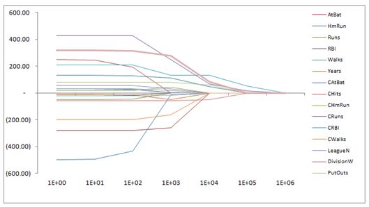
Recall that for ridge regression, as we increased the value of lambda all the coefficients were shrunk towards zero but they did not equal zero exactly. The profile of the coefficients for different values of lambda are shown in the graph below.

If we run the LASSO model on the same dataset please notice that some coefficients are set exactly equal to zero.

This is what we mean when we say LASSO performs feature selection. For a particular value of lambda we are likely to set some coefficients directly to zero. This is a result of the l1 penalty that we impose on the parameters. In below graph on the left we see the contour graph of the SSE (the red ellipses) and the feasible solution set is inside the diamond. Notice that when the solution is at the corner one of the features is equal to zero. In the graph on the right we see the same SSE contour plot but the ridge regression constraint is a circle. It is unlikely that the solution touches an axis where one of the coefficients is zero. The same argument extends to more than two dimensions. This is the reason why LASSO “selects” features.

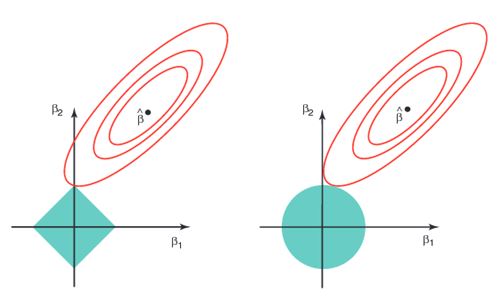
It is important to mention that when features are highly correlated some of them may be set to zero in the LASSO mode. The choice of which feature is retained is arbitrary since the model has no way to distinguish which feature is “best”. In case of ridge regression, both features would be retained with their coefficients shrunk and likely set equal to similar values. The chart from above was taken from Introduction to Statistical Learning and is highly recommended http://www-bcf.usc.edu/~gareth/ISL/.

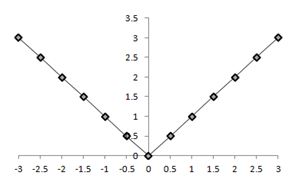
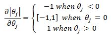
Another important point to note is that the introduction of l1 penalty in the SSE function means we cannot derive a closed form solution for the value of the coefficients. Remember that in OLS and ridge regression we can derive the derivative of the SSE function with respect to the theta coefficients and then set them to zero to arrive at the coefficient values that minimize the SSE function. With the l1 penalty term the derivative is no longer defined. In the graph below we can see that the derivative in the second quadrant is equal to -1 and is 1 in the first quadrant and is undefined at 0.

This means we need to use numerical methods to solve for the coefficients. There are many algorithms to solve this problem but the one I will present is called the coordinate descent algorithm.

Least Squares Cyclical Coordinate Descent:

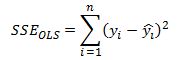
First let us consider the least squares problem and how we can use coordinate descent to solve for the theta coefficients. Remember that in OLS the SSE is given as:

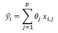
where y hat is equal to:

Therefore:

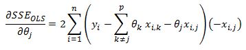
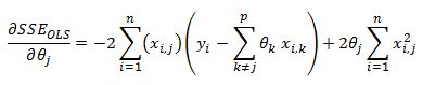
We first take the derivative of the SSE function with respect to theta j

We can strip out the jth parameter out of the sigma summation as:

On the right hand side the sigma summation is done over all values of k to p where k does not equal to j. Using this notation we write the derivative as:

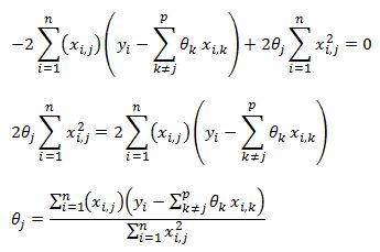
We can take the theta parameter outside of the brackets after some algebra.

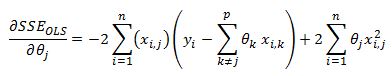
Now notice that the theta coefficient does not depend on i so it can come outside of the summation

We can now set this function to zero and solve for theta j

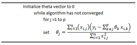
In the cyclical coordinate descent algorithm we step through all of our theta coefficients and update each theta using above equation. It can be shown that this procedure will converge to the global minimum of the SSE function.

The pseudo code of the algorithm is below:

I just want to highlight something about our derived theta update formula

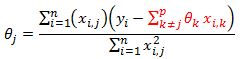
Notice that the formula highlighted in red is the estimate of our model that excludes the impact of feature j. The value inside the bracket is the residual of our model that does not include feature j.

LASSO Cyclical Coordinate Descent:

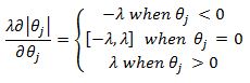
Now we must deal with the nasty l1 penalty term in our SSE if we wish to derive the coordinate descent algorithm for the LASSO model. The derivation is similar to what was presented above except we now have an additional term that we cannot differentiate. We can however use what are known as subgradients. For the absolute value function a subgradient is given as:

Including the lambda term we have:

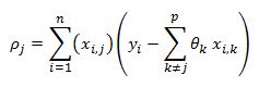
Before we combine the above result with our derived results for least squares derivatives lets define:

and

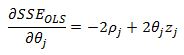
from least squares SSE we already derived:

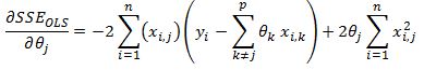
with our new notation we have:

now adding the l1 subgradient we have:

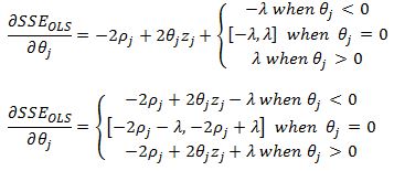
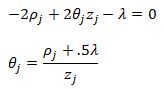
Lets consider case 1 where theta j is less than zero. We have:

Since z is always positive, for theta to be less than zero we must have:

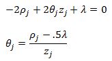
For the third case, following the same logic, we can see that in order for theta to be positive we must have:

And for the case where theta equals zero we need zero to be bounded by the interval:

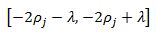
this implies:

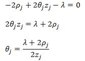
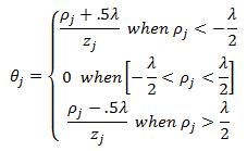
We can finally put the results together. For case 1 we will have the theta update rule:

For case 2 we will set theta equal to zero. And finally for case three we have:

To write it more compactly we have the following theta update rule:

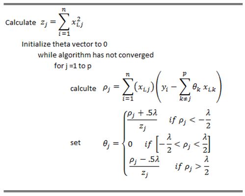
The pseudo code for the coordinate descent algorithm for Lasso is below

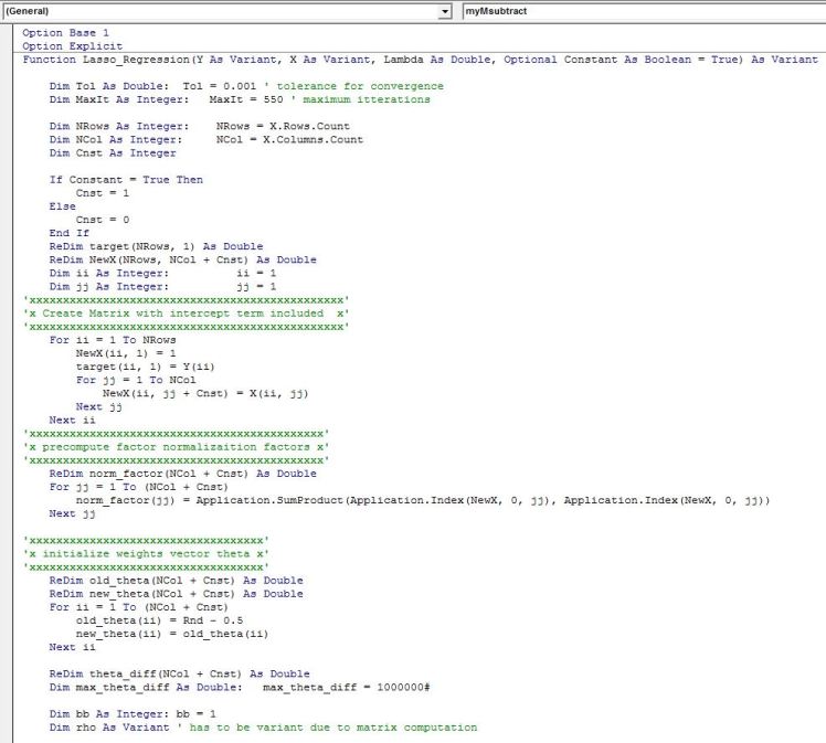
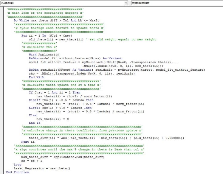
VBA implementation:

Below is the VBA implementation that works similar to Ridge regression function I discussed in a previous post. The output is a row vector of coefficients in the same order as the input of the features into the function.

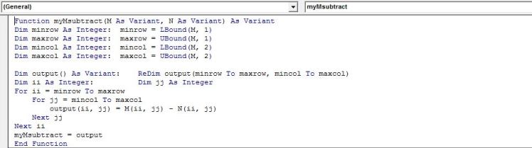
Helper function to calculate matrix subtraction

Some Useful Recourses:

1) Introduction to Statistical Learning by Gareth James, Daniela Witten, Trevor Hastie and Robert Tibshirani. A fantastic book. One of my favourites. Has a good discussion on penalized regression. One of the authors is the originator of the LASSO. Some of the authors have contributed R packages that implement Lasso and also Elastic Net model (a hybrid between ridge and lasso model) www-bcf.usc.edu/~gareth/ISL/

2) Coursera course on regression models http://www.coursera.org/learn/ml-regression. You get hands on experience implementing models in Python. Emily Fox of University of Washington does a fantastic job. The course includes derivation of Lasso and one of the assignments involves coordinate descent algorithm.