In my previous post I showed a coordinate descent algorithm for solving Lasso coefficients. Lasso model is part of a family of penalized regression models that are popular in machine learning and predictive modeling. In today’s post I want to show you how this model can be used to estimate the monthly average price of Aluminium (Ali) 3month forward contract that trades on the London Metals Exchange.

There are a lot of features (independent variables) that are candidates for inclusion into a regression model. As I previously wrote, Lasso performs feature selection via the l1 penalty that is selected outside of the model calibration algorithm. Lambda is a hyper-parameter (or tuning parameter). This parameter is selected via cross-validation techniques that are very simple to implement with R’s glmnet package.

Initial Feature Candidate Set:

To narrow down our initial feature set we should consider what are some of the fundamental drivers of Ali. Via LME’s webpage (link at the end of the post) we can see that transportation and construction accounted for 50% of consumption of Ali in 2011.

More than half of Ali production was in Asia.

Because Ali is light and conducts electricity well it is widely used in the auto industry (body panels and engine blocks), in wiring, kitchen utensils, and in packaging (pop cans). Ali’s use in the auto industry is a promising growth area.

So with that lets have a look at some candidate features. I think a fair place to start is with the world’s largest auto market by sales. Below is the log monthly China auto sales. I also included a Hodrick Prescott (HP) filter and the monthly average Ali 3mth futures price (also in natural log terms). The second chart below is the average Ali price versus cyclical component of the features’ time series (ie deviation from HP trend).

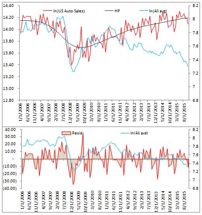
I would suggest that inclusion of US also makes sense since it is the world’s second largest auto market. Below is a similar pair of charts. There appears to be a strong relationship up to 2012 which subsequently disappeared.

Since China has been such a major player in the commodities markets I think it is best to include Chinese Ali imports as a candidate feature in our model. Below is a plot of the data for quick inspection.

I will also include the world total aluminium production as a feature. The plot is below and I also include regional breakdown for the curious (source: http://www.world-aluminium.org/statistics)

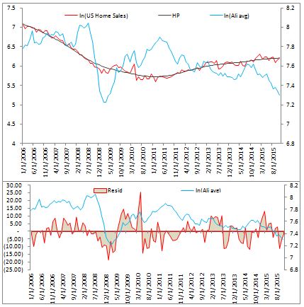
Additionally, since construction is a major component of Ali consumption we can consider US housing construction data as a possible predictive feature.

Since Ali is priced in US dollars, USD value will drive the cost of Ali consumption globally. We can include the monthly average DXY index in the model.

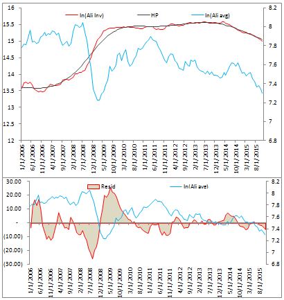
And finally, world Ali inventory should be considered as a feature. Below are the plots.

For our feature set we can use the natural log of each time series and the cyclical component (residual) after running our HP filter. In this specification, the model can learn weights for the raw log time series and the cyclical component. In total, this leaves us with a set of 14 features in the model.

Before we proceed I first want address an issue a reader may take with my choice of using the features’ raw price time series and the cyclical component as input variables. The reason for the choice is that by our definition we have feature level = HP trend + cycle. This can be written as HP trend = feature level – cycle. Therefore in our model we are allowing for the trend component to be used as a feature. What I mean by that is we will have beta1*feature level + beta2*cycle. If our estimated coefficient parameter vector is [1,-1] then our model selected HP trend as a independent variable. Alternatively we can have the vector [0,-1] which means the model has selected the cyclical component as an independent variable. The estimated beta vector can be fitted without constraints and therefore the model can learn on its own without our guidance. We try to control for over fitting via our lambda parameter and leave the rest in the model’s hands without constraining (ie biasing) the model.

Model Estimation:

First let’s have a peek at the correlation matrix.

We can see that Ali inventory has a large negative correlation with US home sales. Also, inventory data is positively correlated with Chinese auto sales. There are few strongly correlated clusters so we can expect Lasso to retain many of the variables if they have predictive value. In cases of strong correlation, Lasso will drop some of the features it considers redundant or those that have no predictive value.

But enough of descriptive statistics, lets estimate the model. Our first step is to select an optimal lambda penalty parameter. This can be done using cross-validation techniques. R’s glmnet package performs 10-fold cross validation. As I discussed previously in my Ridge regression post, when we are fitting a penalized regression model we need to standardize our data so that it is on the same scale. This is obvious when we remind ourselves that we are minimizing below function

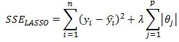
To ensure that no feature dominates the second term in the above equation we need to normalize the features.

We can now run cross-validation to estimate the best lambda parameter.

We can see that a lambda value of .00013862 returns the least mean squared error on our cross-validation run.

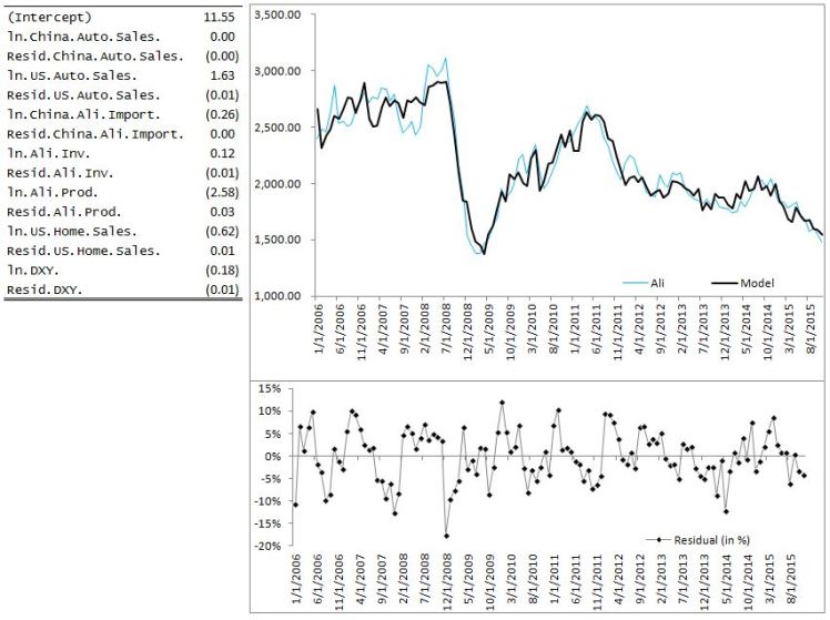
With this value of lambda our estimated coefficients are:

In the Lasso model China auto sales coefficient has been set to zero. Many of the cyclical features have also been shrunk close to zero but not set exactly to zero.

And that is all there is to estimating a Lasso model in R. To plot the fitted values against the average monthly Ali price we simply take the exponent of the fitted estimate and we are done!

Final Note:

Notice that I did not perform any statistical inference on the coefficients. We are not trying to establish causality effects or to analyze marginal impact of a particular feature on the price of Ali. We are simply using a predictive model that fits the data well given a set of features that were chosen a priori. This approach can be criticized in many ways but I should also mention that penalized regression models do have their place in a modeller’s arsenal. The Lasso model can be used to prototype a model for a particular asset quickly and can help with feature selection.

Useful Resources:

1) A dated but interesting article from FT http://www.ft.com/intl/cms/s/0/7c671aac-4372-11e4-be3f-00144feabdc0.html#axzz3wQXAdf92

2) World Aluminium production statistics http://www.world-aluminium.org/statistics

3) LME Aluminium production and consumption page http://www.lme.com/en-gb/metals/non-ferrous/aluminium/production-and-consumption

4) A vignette on R’s glmnet package https://web.stanford.edu/~hastie/Papers/Glmnet_Vignette.pdf

5) Discussion of Hodrick Prescott filter https://quantmacro.wordpress.com/2015/06/25/hodrick-prescott-filter-in-excel/