I recently went through a Coursera course on Classification taught by Carlos Guestrin from U of Washington and thought it was excellent.   There was an interesting discussion on model overfitting that I thought I would share. In previous posts I discussed linear models with shrinkage parameters such us ridge and lasso regression models. Similar approach should be applied when building a classifier to reduce model complexity. I previously posted on logistic regression and wont discuss the model here.  Instead, I want to echo what was discussed by Carlos in the Coursera course.

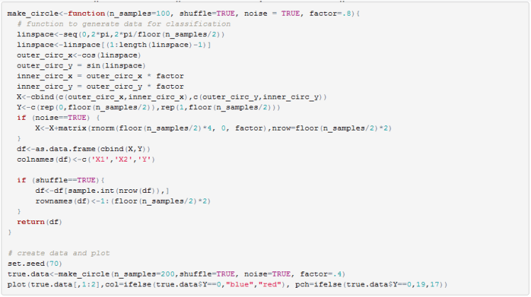
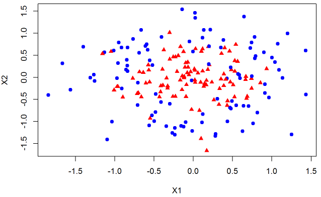
First, we need some data to play with. I wrote a function that is similar to Python’s make_circles function. I classify the points in the inner circle as class 1 and the outer circle as class 0. I also generated noise so that the data is not separable. We will work in two dimensions because visualization provides a key insight.

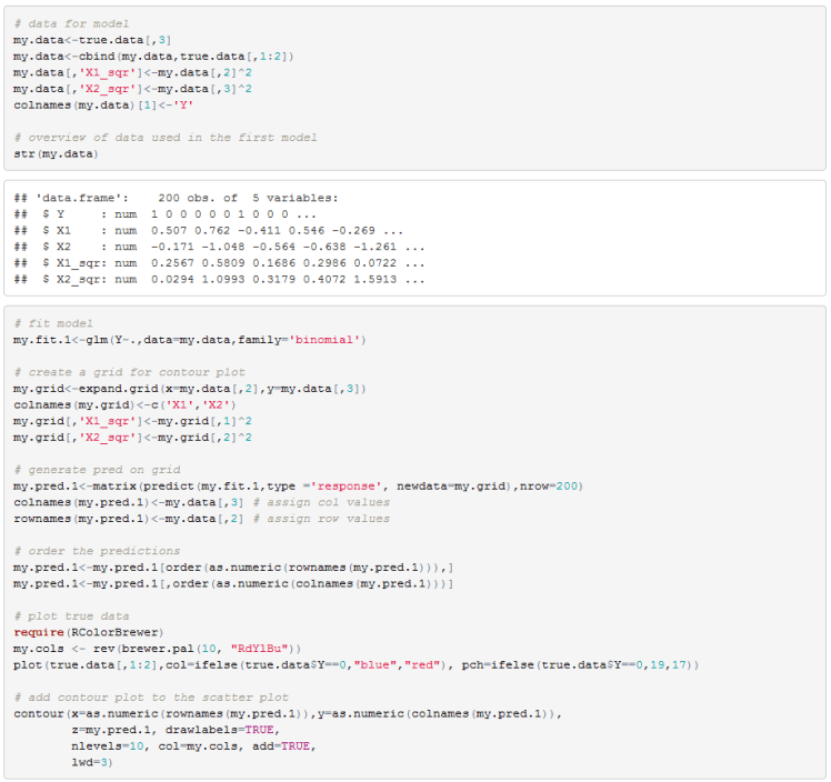
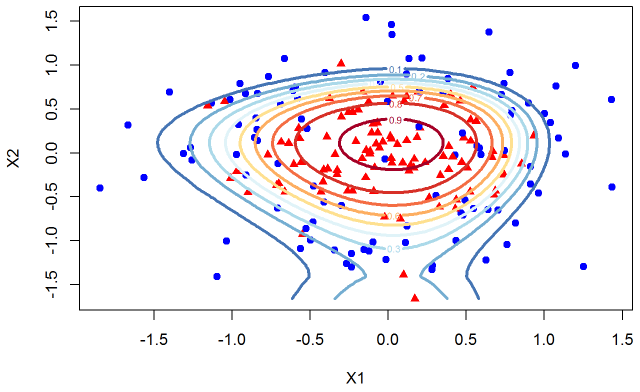
Since we know the true model we can estimate a logistic classifier using X1, X2, and their squares. I also include a contour plot of the fitted probability. The contour plot gives a probability, given an X1 X2 pair, of being in the inner circle (ie a red triangle). Often a single decision boundary is drawn using a fixed classification threshold but here we want to see decision boundaries for a variety of thresholds.

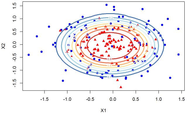
If we were to use a .5 threshold we would consider the yellow line as the decision boundary. Any point inside the yellow circle would be classified as a triangle while any point outside the yellow circle would be classified as a blue circle.

Our data is not separable so we expect the model to make misclassifications. Overall the fit seems reasonable. In real world we do not know the true distribution of the data so we often have to add features to the model to improve the fit (decrease misclassification rate or increase AUC or any other metric). Lets continue with this dataset but engineer more features from X1 and X2 to see the impact on the decision boundaries.

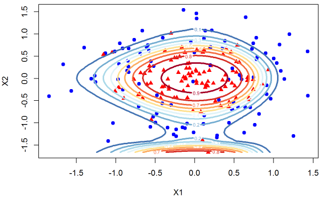
In the next step I add more features with X1^3 and X2^3. You can see the decision boundaries below.

The contour plots are distorted to capture the idiosyncrasy of the data sampled. Lets carry on the exercise and add X^4 terms.

And lets now include X^5 terms.

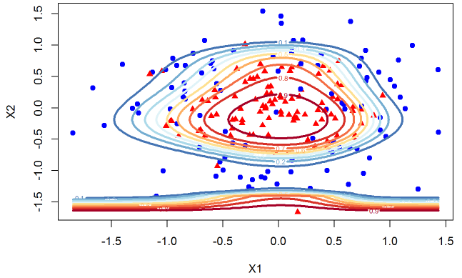
You can see that the model has a very unnatural shape. Since we know the true data we can very clearly see that we are overfitting.   I hope you agree that it is a useful exercise to be able to see the dynamics of the contour plots as we overfit the data but in the real world we are working with much higher dimensions so we cannot observe the decision boundaries. But the main point that I want to share with you is something that escaped me until I took this course. Look at the change in the probabilities that we assign to class 1 as we overfit the data. It is helpful to see the plots next to each other. The left plot is the model that only uses X1, X2, and their squares. The model on the right has X1, X2, X1^2, X2^2,… X1^5, X2^5 as its features.

Notice that for the overfitted model on the right we go from .1 to .5 probability for a much smaller change in X2 than for the model on the left. This means that as we overfit the data we not only chase idiosyncratic point we are also decreasing the measure of uncertainty about our classifications. For small changes in X2 our probability of classifying a data point to one of the classes changes rapidly. So there are two effects here, one is that we overfit the data and in general our decision boundaries have incorrect shape. Secondly, where the data is clustered and the model is overfitting it will overstate the uncertainty with a steep probability surface (decision boundaries are too close together).

As you probably already guessed, to avoid the issue of overfitting we can introduce a shrinkage factor similar to what we did for linear regression in my previous posts.   I thought about implementing this in excel since I previously posted about logistic, ridge, and lasso regression implementation but decided not to spend the time. R’s glmnet package has these models implemented and any serious user will need to cross validate the shrinkage coefficient so I felt there was little benefit to implementing this in VBA.

As just mentioned, R’s glmnet package has all the functions needed to perform cross validation to calculate the shrinkage factor lambda.

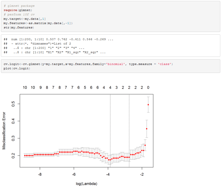
I used misclassification error rate as the selection criteria for the lambda parameter. Cv.glmnet performs 10-fold cross validation as the default which suits us here.

I used a lambda coefficient that is within 1 standard deviation of the absolute low.

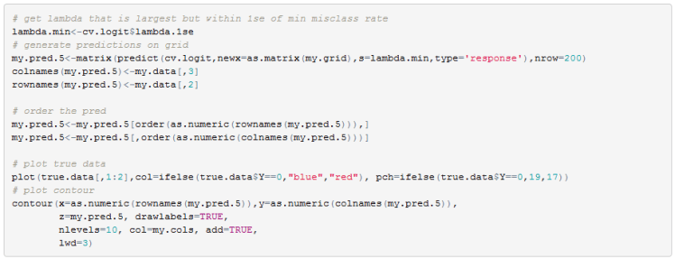
Looking at the contours plot of the probability surface we can see that we get back to very nice decision boundaries. Remember that we used all the higher order features when performing cross validation and yet the model selected only those that perform the best in a cross validation run.

Hope you found this as useful as I did. There are many models put out by broker researchers that use classifiers to work out the probability of a recession, or a probability of a drawdown in a particular asset class. If you are one of the people who uses such models hopefully you gained some insight from this discussion. I know that I have to come back to my models and check for overfitting and most likely recalibrate.

Useful Resources:

• Machine Learning: Classification on courser https://www.coursera.org/learn/ml-classification/
• R’s Glmnet vignette https://web.stanford.edu/~hastie/Papers/Glmnet_Vignette.pdf
• My previous post on Lasso https://quantmacro.wordpress.com/2016/01/03/lasso-regression-in-vba/
• My previous post on Ridge https://quantmacro.wordpress.com/2015/12/11/ridge-regression-in-excelvba/
• My previous post on Logistic regression https://quantmacro.wordpress.com/2015/07/06/logistic-regression-in-vba/